Full FEM is the direct 3D simulation of the borefield: instead of a g-function and its superposition, the ground mesh is stepped in time with the project's actual loads, and the boreholes and the groundwater can carry their own dynamics. It answers questions that a step response cannot: how the heat stored in the fluid, the pipes and the grout buffers hourly peaks and load or pump stops, what happens when the flow of the groundwater follows from heads, wells and layers, and how cold, heavier and more viscous water changes that flow. Like the 3D analysis it checks a chosen design; Calculate, the optimisation and the studies stay with the analytic model, and a separate command sizes the length with the direct model.
23.1 Four combinations of ground and borehole physics
Two independent choices on the Full FEM page (Physics & run) give four combinations. In all of them the ground is transient; "steady-state" refers to the borehole interior, which is then in equilibrium at every step.
| Ground model | Steady-state boreholes | Full transient boreholes |
|---|---|---|
| Simple (conduction, optional prescribed horizontal flow) | ground stepped with the actual loads; borehole as resistance | ground and borehole columns (fluid, pipe walls, grout) stepped together |
| Fully coupled thermo-hydraulic (TH) | head and temperature iterated in every step; borehole as resistance | head, temperature and borehole columns, committed together |
A direct run computes no g-function. It keeps the requested power, the power delivered through the borehole walls, the loop power, the heat stored in the boreholes and in the ground, inlet, outlet and mean fluid temperatures with their extremes within each output interval, series per borehole, the heat through every group of faces, and the energy, loop and water balances.
Loop control. Exactly one control closes the loop:
- wall power: the loads are the heat rate through the borehole walls, the meaning of every load input of the design (the ground load);
- loop power: the loads are the heat delivered by the fluid loop, , for example a heat pump's evaporator; the borehole storage lies between loop and wall;
- inlet temperature: a time series of is prescribed and the powers are results (thermal response tests, performance tests).
The automatic setting takes loop power with transient boreholes and wall power with steady-state boreholes, where the two are the same. With the pump off the borehole exchange with the fluid stops, and a load requested during that time is reported as undelivered energy instead of being forced through.
23.2 Ground, materials, initial and boundary conditions
The ground uses the mesh rules of the 3D analysis with the same end time, so both paths run on identical meshes. The unknowns are the perturbation against the initial temperature: by default the undisturbed geothermal profile , alternatively the project's mean ground temperature or a uniform value. An optional spin-up lets the background evolve without loads before operation starts.
The faces of the block are thermally Initial (held at the initial temperature, the default), Zero flux, or, at the bottom, Geothermal flux; water entering the block carries the initial temperature of the face or a given inflow temperature. Initial and boundary conditions must agree (a geothermal bottom flux needs the geothermal profile, for example), otherwise the run is refused with a message.
Materials. The direct modes take the ground properties of each layer from the Materials page: the Ground page values (the default, so the 3D run and the 2D design use the same ground), bulk values with an anisotropic conductivity, or the solid matrix plus the porosity. With local thermal equilibrium between solid and pore water,
with the porosity of the layer and the conductivity of the pore water (default 0.58 W/(m K)). The geometric mean lies between the series and parallel bounds and is the usual estimate for saturated granular rock (Woodside & Messmer 1961). Example: = 3.0, = 0.58 W/(m K), = 0.25 give = 1.989 W/(m K); = 2.0 and = 4.18 MJ/(m³ K) give = 2.545 MJ/(m³ K). Values that were pre-filled and not edited are marked as assumed on the page and in the results.
Anisotropic conduction uses the tensor . With the scaled depth the anisotropic equation becomes isotropic with , so the mean wall temperature of a vertical borehole is the finite line source with and the length and depth divided by (in the form of Claesson & Javed 2011). For a 40 m borehole with = 2.5 and = 0.8 W/(m K) over 3 years, the effect of the anisotropy on the mean wall temperature is 0.276 K on hexahedra and 0.283 K on tetrahedra against 0.284 K from the scaled line source.
23.3 Time stepping, peaks and outputs
Each step is a backward Euler step of the ground with the lumped capacity,
( the constant terms of the initial temperature in the borehole couplings, the distribution of the field heat rate ). The system is linear in , so a prescribed inlet temperature gives in closed form from one extra solve.
Adaptive steps on a ladder. The steps are , at most 30 days, so that every pair of configuration and step size is factorised once and reused. The error of a step is estimated by step doubling (one step of against two of ) on the ground temperatures and on the mean fluid temperature (steady-state boreholes) or the mean wall temperature (transient boreholes). Above the tolerance the step is rejected and halved; at or below a quarter of it the next step doubles. After every change of the input (load, flow, pump on or off) the step restarts at the initial step (1 h by default, the rung 32 min), and every event is hit exactly. The default tolerance is 0.01 K per step.
Peaks. The monthly peak loads of the classic monthly method are run as trial branches: from the accepted base state at the start of the peak the peak replaces the base load until the month end, and the extreme fluid temperature of the branch is the peak result. A branch never enters the operational history. For the same response, linear superposition makes this identical to the peak formula of the design.
Outputs. The output resolution is separate from the solver's: each accepted step contributes to every output interval it overlaps. Means are time means; the lowest and highest values come from the solver steps (and, with transient boreholes, from their sub-steps). The ground temperature is stored at month ends for the 3D view, the maps and the export.
Energy. Per accepted step , with the heat leaving through the faces by conduction and advection; the relative residual of a step is below .
23.4 The near-borehole model
A borehole is a line of mesh nodes. The well index, with the calibrated constant and the axis cell , couples the wall to the line node and is exact for the steady field around the axis. In a time-stepped run the borehole wall temperature is needed at every step, and at short times the node coupling lags far behind: the heat of a step enters the lumped capacity of the whole axis cell instead of the thin annulus at the wall. For 30 W/m in a ground of 2 W/(m K) and 2.4 MJ/(m³ K), = 75 mm and an axis cell of 0.715 m:
| Time | True wall rise (cylinder source) | Error of the well index | Error of the optimal ring, |
|---|---|---|---|
| 1 h | 1.51 K | −1.20 K | −1.41 K |
| 6 h | 2.84 K | −2.11 K | −2.24 K |
| 24 h | 4.20 K | −2.22 K | −2.15 K |
| 7 d | 6.37 K | −0.62 K | −0.50 K |
| 30 d | 8.08 K | −0.09 K | −0.08 K |
The error decays over the validity time ( the axis cell; 6.1 days for 0.715 m), which the mesh summary reports per borehole. A finer axis cell does not help a node coupling. The same holds for the optimal nodal distance of Diersch et al. (2011, Part 2): with nodes on a regular polygon around a borehole node the node temperature equals the wall temperature for a distance with
On the hexahedral grid the counterpart is the square axis cell , where the well-index correction is zero by construction. This optimal ring is selectable for runs that are to be compared with codes built on that principle; it changes the axis cells only and does not remove the short-time lag.
Radial sub-grid (default). Every line point carries a one-dimensional axisymmetric finite-volume model of the ground from the wall to a coupling radius : 30 cells spaced geometrically, the wall heat rate entering at the inner node, and at the ring temperature, the mean of the mesh temperature at 16 points on the circle of radius around the axis. The mesh error from the line source is confined to about one cell around the axis, so the ring sees the correct field at all times. For a step of length the wall temperature at its end is affine in the step's wall heat rate and ring temperature,
with , depending on the step size only (two unit responses per radial grid) and on the accepted sub-grid state. The heat still enters the ground mesh at the line point: the sub-grid is a local refinement of the temperature between the wall and , it adds no heat and no resistance, and the energy balance of a run is that of the mesh. For long steps and , the steady radial resistance. Near a neighbouring axis is reduced; below 1.4 cells the point falls back to the well index, with a note.
Against the cylinder source superposed in time, the sub-grid follows short pulses and their recovery within 0.07 K (the well index: up to 2.3 K at 30 W/m, 3.9 K at 50 W/m), is converged in the ring radius, the radial cells and the sub-steps, and approaches the steady well index at long times. It is conductive: a local Péclet number above 0.5 is reported.
23.5 Full transient boreholes
With full transient boreholes the fluid moves through the pipes with its transit delay, and the fluid, the pipe walls and the grout store heat. The steady borehole, , is the limit of vanishing capacities.
23.5.1 The borehole column
Every string of the borehole network (its stages in flow order) becomes one one-dimensional transient model, the column. Its axial cells (about 1 m, automatic) carry the fluid channels and the fixed nodes of the TRCM cross-section (Bauer et al. 2011): for a single U-tube one fluid node per leg and one grout node per leg; for a coaxial pipe the inner pipe, the annulus, the grout and the inner pipe wall. The capacities are
- fluid per channel;
- grout per grout node, with the grout annulus without the pipe cross-sections;
- pipe walls (default 1.8 MJ/(m³ K) for PE), placed at the one fixed node each wall belongs to, so that nothing is counted twice.
The wall node is the inner node of the radial sub-grid. The fluid is advected by upwind finite volumes along each flow path (leg down, U-turn, leg up; series stages by passing the outlet on, parallel stages through a mixing node), with the exponentially fitted exchange of the steady element, so that the column at vanishing capacities is the steady heat exchanger exactly.
23.5.2 Multirate stepping and the monolithic coupling
The ground needs steps of hours to days; the fluid transit through a 150 m U-tube takes minutes. The column is therefore advanced in sub-steps inside each ground step: after a change of the input the sub-step is the transit time divided by 40 (between 0.5 s and 300 s) for three transits, then it doubles to the end of the step. The column is linear in its inputs, the ring temperatures and the field inlet temperature, which are held at their values at the end of the ground step. The step-mean wall heat of every point is therefore affine,
with unit responses and that depend only on the step size and the sub-step pattern (cached with the factorisations) and a history response of the stored state. One ring unknown per line point is added to the ground system and enters the ground rows of the point; the global system is then solved once per ground step with the borehole internals condensed onto the rings. Because the ground receives exactly the column's integrated wall heat, the balance
holds to round-off per step and over the run.
23.5.3 Controls with storage, pump stops and flow reversal
Under loop power the outlet is affine in , so follows in closed form per step and the storage buffers the wall heat. Under wall power the closure is an inverse problem: a step much shorter than the borehole time constant would need large swings of to push the requested heat through the capacities. The control therefore holds over at least the control interval
( the heat capacity per metre of fluid, pipe walls and grout), and shorter load intervals are merged. Each distinct flow state (pump on at a binned flow and direction, or off) is a configuration with its own matrices; the column state is carried across configurations. With the pump off the fluid stands and the stored heat relaxes into the ground; at restart the stored fluid leaves the outlet first. A flow reversal swaps the roles of the legs on the same state layout. All boundary conditions of the design map onto the same columns.
23.6 Saturated groundwater flow
The fully coupled TH ground computes the groundwater flow itself: saturated, single-phase flow with local thermal equilibrium between rock and water; the closed-loop boreholes add heat, no water. With the hydraulic head ( the gauge pore pressure, the elevation, the reference density) the mass balance and Darcy's law read
with the specific storage, the porosity, the thermal expansion of the water (the term vanishes for a constant density), the well sources, the permeability tensor, the downward unit vector and the Darcy velocity (the volume flux). The water laws are a constant or linear density and a constant, exponential or Vogel viscosity,
(pure water, 0–100 °C, within about 2 %). With a constant density a hydrostatic state has zero flow to round-off. The equations are discretised by the Galerkin method on the same mesh, with lumped storage and backward Euler; the hydraulic data are taken per layer and never mixed into effective values.
Boundary conditions. Each face is No flow, Prescribed head (the reference head at the field centre plus a regional gradient along a given direction, hydrostatic in depth) or Prescribed flux. The default is the water table at the surface, head-controlled sides and a no-flow bottom. Wells are line sources over their screen with a given rate and temperature. The initial state is the hydrostatic rest or the steady flow of the conditions; Compute groundwater flow shows the background flow and its water balance before the long run.
Conservative fluxes. Every element matrix has zero row sums, so the Galerkin equation of node is the water balance of its control volume, with the node-pair fluxes
( the boundary inflow, the well rate, the storage rate). The balance holds per node to the solver tolerance, and these fluxes are what carries the heat in the transport.
From a Darcy velocity to a head gradient. A prescribed Darcy velocity of the Ground page can be converted into the regional head gradient that carries the same discharge over the active depth,
with the overlap of layer with the active depth and its hydraulic conductivity along the flow at the mean ground temperature. A homogeneous ground gets exactly. The coupled ground refuses a prescribed velocity, because the flow is a result there.
23.7 Heat transport with computed flow
The heat transport of the coupled ground is the advection–dispersion equation
with the conductivity of the saturated ground, the thermal dispersion with the longitudinal and transverse dispersivities , (default zero) and the streamline diffusion. A temperature front drifts with the heat-transport velocity .
Conservative advection. The advection uses the node-pair water fluxes of (23.11) in the advective form: row receives plus the inflow of water at the face or well temperature, with the mean of the two nodes. A uniform temperature is then an exact steady state whatever the flow, and the global sum telescopes to the boundary terms when the water balance closes. For a divergence-free prescribed velocity this form equals the Galerkin advection exactly, so the transport ground reproduces the simple ground with prescribed flow to round-off.
Stabilisation. The default is the streamline diffusion of (22.12) generalised to 3D flow, anisotropy and dispersion; it is symmetric with zero row sums, never adds or removes heat and acts only along the flow. An exponentially fitted edge upwinding (monotone wherever the pair conductance is positive) and plain Galerkin are available for verification. On a front moved 8 m with = 0.1 m, the two stabilised forms stay within the bounds to round-off up to an element Péclet number of 25, while Galerkin overshoots by 0.18 % at 5 and 1.5 % at 25. The mesh is not refined to cap the Péclet number (in a 1 m/d aquifer that would need cells of about 2 m); the largest element Péclet number and the volume above 2 are reported instead.
Faces and truncation. The heat leaving the block splits exactly into face groups (the sides, the bottom, the top, the wells, the background drift and the water entering storage). When the heat through the sides and the bottom exceeds 5 % of the borehole heat, a note asks for a larger block. The mesh is extended downstream by the drift estimated from the regional head gradient before the flow is computed.
23.8 Two-way thermo-hydraulic coupling
The water balance uses the reference density for the volume and only in the buoyancy and, through , in the expansion of the stored water (the Boussinesq form). One backward Euler step from the accepted state is an iterated staggered (Picard) solve; with the iteration repeats
- the water properties , per element at the mean temperature of its nodes, from , and the hydraulic step to the head (optionally under-relaxed);
- the node-pair fluxes of and the transport operator of the new flow;
- the thermal step of the ground with the borehole couplings and the loop control, giving .
An iterate is converged when the temperatures change by less than K (plus relative), the pressures by less than 1 Pa (plus relative), and the hydraulic equations of the new temperatures hold to a relative defect of . The energy balance of a step closes for the operator of its last thermal solve, whatever the iteration count. With constant water laws the flow does not depend on the temperature and one iteration is exact.
A step that does not converge within 25 iterations is rejected and repeated with half the step, and nothing of it reaches the accepted state or the balances; after six failures in a row the run stops with a message. Two measures reduce the work without changing the converged solution: Anderson acceleration of depth 3 (Walker & Ni 2011) of the temperature fixed point, which halves the iterations of strongly coupled steps, and a lagged flow that reuses the last converged flow as the first iterate when the temperature has changed by at most 0.5 K. With full transient boreholes the column unit responses do not depend on the ground and stay valid for every iterate; ground, head and column states are committed together only after the coupling has converged.
23.9 Sizing with the 3D model
Size with 3D is a separate command on the Physics & run page. It sizes the mean borehole length with the selected direct model, the positions fixed and unequal lengths scaled in proportion. Every trial length is a full direct run from the freshly initialised ground; no g-function or cache stands in for it. The search starts at the 2D size, brackets the root of the limit violation in steps of 15 % and refines it with Brent's method (Brent 1973) to the larger of the tolerance and 0.5 m, with at most 16 runs. The results page also states whether the 3D model changes the feasibility of the 2D design against the limits.
23.10 Examples
23.10.1 Transient boreholes: peaks and a pump stop
One 50 m single-U borehole ( = 75 mm) in 2.0 W/(m K) ground at 10 °C, flow 0.4 l/s, loop-power control, an hourly series: 2.5 kW extraction for 6 h, 18 h of circulation without load, a second 6-hour peak, then the pump stops; one year simulated. The heat capacity per metre is = 4.3 (fluid) + 0.95 (pipe walls) + 32.1 (grout) = 37.4 kJ/(m K); with = 0.109 m K/W the time constant is 68 min. The fluid transit is 10.78 cm² × 50 m / 0.4 l/s = 135 s, so the first borehole sub-step is 3.4 s. In the first hour of the peak the heat pump takes 2.50 kW, but only 1.20 kW cross the borehole wall; 1.30 kWh come from the borehole store. By hour 6 the wall power has risen to 2.33 kW.
| Quantity | 2D design | Full FEM, 0.01 K | Full FEM, 0.003 K |
|---|---|---|---|
| Mean , hour 1 (peak start) | 3.35 | 4.88 | 4.92 |
| Mean , hour 6 (end of the peak) | 0.47 | 0.59 | 0.59 |
| Mean , hour 7 (after the load stop) | 6.84 | 5.42 | 5.37 |
| Lowest within hour 7 | – | 2.58 | 1.23 |
| Mean , hour 31 (after the pump stop) | 6.42 | 4.35 | 4.33 |
| Mean , hour 72 | 9.57 | 9.56 | 9.56 |
| Lowest of the period | 0.04 | 0.03 | 0.01 |
| Lowest inlet temperature | – | −0.75 | −0.77 |
| Time steps accepted / rejected | – | 237 / 5 | 370 / 23 |
The differences lie in the hours around the changes: +1.5 K at the peak start (the store delivers heat first), −1.4 K after the load stop and −2.1 K after the pump stop (the ground refills the store). The hourly means hardly depend on the step tolerance, but the lowest value right after the load stop does: the step-doubling estimate controls the ground and wall temperatures, while the fluid changes within minutes and is held constant over each ground step. Hourly values and the first interval after a stop therefore need a tolerance of 0.003 K (here 1.5 times the run time).
23.10.2 Coupled TH ground: a borehole in an aquifer
One 40 m single-U borehole ( = 55 mm) in a sand-and-gravel aquifer ( m², ground 2.6 W/(m K), 9 °C at the surface), top and sides with prescribed head and a regional gradient of 0.00044, a no-flow bottom, steady initial flow, linear density and Vogel viscosity, full transient boreholes, 1.5 kW extraction for a year as monthly loads, limits 2 … 30 °C, Coarse mesh. With = 1.319 mPa s at the start the hydraulic conductivity is m/s, the regional Darcy velocity m/s (3.1 m/a) and the heat-transport velocity m/s (5.9 m/a); the block is extended 9.8 m downstream.
| Quantity | Value |
|---|---|
| / of the year, 2D design | −5.25 / −2.69 °C |
| / of the year, Full FEM | −5.13 / −2.75 °C |
| Monthly mean , month 1 / 6 / 12 | −1.64 / −4.50 / −5.10 °C |
| Coupling iterations per step (mean / max) | 2.2 / 3 |
| Time steps accepted / rejected | 300 / 4 |
| Water / energy balance (relative) | / |
| Mesh | 13 860 nodes, 12 180 hexahedra |
| Required length: 2D / Size with 3D | 75.95 m / 75.13 m (4 runs); at the 3D length 2.01 °C |
| With ten times the permeability: Darcy velocity, | m/s (31 m/a); −2.92 °C |
At 3.1 m/a the flow brings heat to the borehole slowly: after one year the 3D run is only 0.12 K warmer than the 2D design (flow and borehole storage together), and Size with 3D needs four runs to find a length 1.1 % shorter than the 2D size (75.95 m feasible, 66.04 m too short, then 75.13 m and 74.88 m by Brent's method). With ten times the permeability the water replaces the heat taken, the temperature levels off after about three months, and the groundwater becomes the deciding factor of the design. There the element Péclet numbers reach 25.6 (91.7 % of the volume above 2) on the Coarse mesh: the solution stays bounded, but the plume is smeared, and a design should be repeated on the Medium mesh.
23.11 Verification
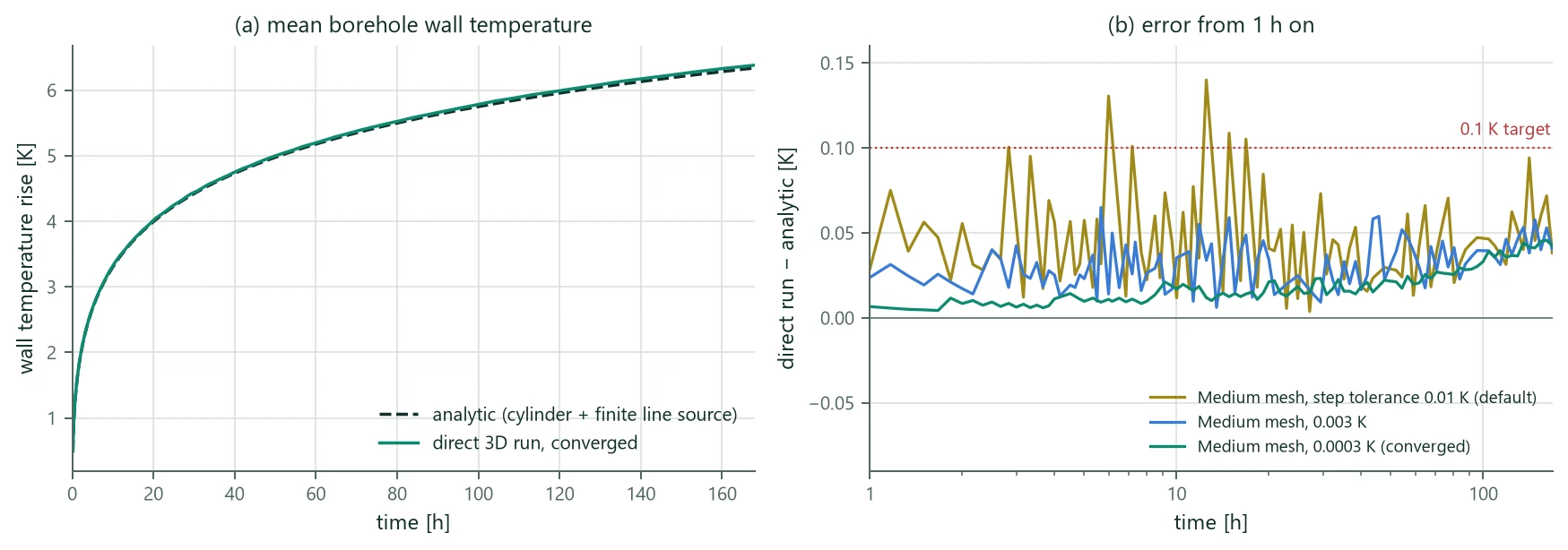
The assembled program was verified case by case against independent references: analytic solutions computed separately (the cylinder source at the wall combined with the finite line source and its mirror image, and with groundwater the moving finite line source of Molina-Giraldo et al. 2011), the program's dynamic borehole model run at two resolutions, measured data, and an independent finite-element code. Each case was run on a convergence ladder (Coarse, Medium, Fine; step tolerances 0.01 to 0.0003 K; the domain doubled). The target after convergence is 0.1 K for temperatures, 1 % of the scale for head and Darcy flux, and 0.1 % of the throughput for the cumulative energy and water balances.
| Case | Reference | Converged result | Default settings |
|---|---|---|---|
| single 50 m borehole, 30 W/m, 7 days hourly and 1 year; simple ground, steady boreholes | cylinder + finite line source | wall temperature within 0.049 K (week and year) | 0.14 K (week), 0.092 K (year) |
| dense 2 × 2 field at 1.5 m | superposed analytic | 0.053 K (week); dense-field warning | 0.14 K; Coarse 2.3 K (sub-grid falls back to the well index in the gap) |
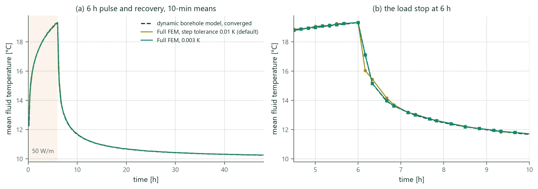
| transient boreholes: 7 days at 30 W/m; 6 h pulse of 50 W/m and recovery | dynamic borehole model | fluid within 0.091 K (week), 0.043 K (pulse); inlet step reaches the outlet after 1.025 transits | 0.10 K (week); 1.08 K in the first 10 min after the pulse |
| sandbox thermal response test of Beier et al. (2011), 52 h, measured inlet | measured outlet | RMSE 0.162 K, bias +0.16 K | the same |
| groundwater m/s, −30 W/m, 1 year; prescribed and computed flow | cylinder + moving FLS | 0.087 K; flow effect within 0.057 K of 0.29 K; computed = prescribed flow within 0.003 K | 0.13 K (Medium) |
| groundwater components: Darcy flow, Theis (1935) drawdown, pressure diffusion, Ogata & Banks (1961) front, dispersion | exact / analytic | exact to ; Theis 0.27 %; order 2.01; front of the drive | – |
| porous cavity at Ra = 100 (Walker & Homsy 1978); buoyant cavity with linear density and Vogel viscosity | published Nusselt numbers; independent FE code | Nu 3.111 (published 3.097–3.141); 0.126 K = 0.6 % of the 20 K drive | – |
| 2 × 2 field of 100 m in an aquifer, coupled TH, one year with peaks | self-convergence | Medium → Fine 0.0007 K; time step 0.011 K; balances | Coarse − Medium 0.055 K |
| 40 m borehole in a buoyant aquifer, coupled TH + transient boreholes, 5 days + pump stop | fine mesh, fixed 15-min steps | reference converged to K | 0.055 K as hourly means; 0.115 K right after the pump stop |
| limits joining the four combinations | exact limits | all within K | – |
| Size with 3D, 40 m, −1.5 kW, °C | 2D sizing | simple = 2D length (75.95 m, 3 runs); coupled TH + transient 75.13 m (4 runs) | – |
Figure 20 shows the single-borehole case: once converged, the direct run follows the analytic wall temperature within 0.05 K from the first hour; the default tolerance stays within 0.14 K. Figure 21 shows the pulse with transient boreholes: the converged run lies on the dynamic borehole model, while the default tolerance misses the drop in the first 10 minutes after the load stop (16.04 °C instead of 17.13 °C) and is back within 0.14 K from 6.5 h on. Mesh, domain and borehole resolution are converged to better than 0.05 K in every case (Medium to Fine at most 0.015 K), and energy, loop and water balances close to or better.
The independent finite-element code with a lumped borehole node lags behind the wall before its validity time (as in Table 39); its ground at 2 m and 5 m from the borehole agrees within 0.01–0.04 K, but before that time it is not a reference for the near field, and the comparisons of the borehole are informative only. No external code couples a two-way TH ground with transient boreholes in one process; the combined mode is verified by its exact limits, by the comparisons of its components, and by a fine-mesh reference of the same equations.
23.12 Limitations
- Step tolerance. The default of 0.01 K per step suits monthly design values. Hourly values and the first interval after a load or pump stop need 0.003 K or tighter (1.3–1.6 times the run time); with 0.003 K the single-borehole week is within 0.07 K and the pulse within 0.05 K. The estimate controls the ground and wall temperatures, not the fluid directly.
- Monthly design loads: transient boreholes change the month-end temperatures little (within 0.017 K of steady boreholes for a 2 × 2 field over a year); the peak trials differ by up to about 1 K because the storage buffers the few-hour peaks.
- Radial sub-grid: a small positive bias of 0.02–0.05 K that grows slowly over months; it is conductive and costs about 0.04 K on the flow effect against the well index.
- Dense fields: with fewer than three axis cells between boreholes, or a gap narrower than about 1.4 axis cells on a coarse mesh, the near field falls back to the well index; the program warns and points to the BTES model.
- Deep coaxial boreholes: for a borehole several hundred metres deep, a homogeneous ground with a conductivity fitted by a line-source evaluation does not reproduce a measured distributed response test to the 0.3 K target, although the result is mesh-converged; the depth-resolved coupling needs a layered ground description there.
- Physics: saturated single-phase flow, no unsaturated zone, no freezing of ground or brine, constant brine properties; the water balance is a volume balance with the reference density. Assumed hydraulic values are listed in the results and should be replaced by site data.
- Cost: the coupled ground costs 14–24 times the run with constant water laws (a 2 × 2 field over a year on the Medium mesh: 815 s against 63 s), every load change needs a new direct run, and Size with 3D needs several full runs. The program estimates the run time before the start (within about 25 % in the verification runs).