 BoreTherm
Monte Carlo
Inspect distributions, quantiles, failure counts and sensitivity. Repeating a seed and sampling method reproduces the same samples. The 100-sample example is an introduction; increase samples and check convergence for a stable tail estimate. Results depend on the assumed distributions and correlations.
Step-by-step workflows · Menus and keyboard
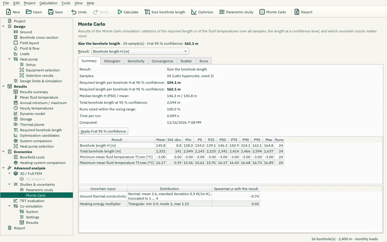
| Control | Meaning / action | Unit | Range / choices | Example value |
|---|---|---|---|---|
| Result: | The result shown in the histogram, sensitivity, convergence and scatter charts. | Borehole length H [m] / Total borehole length [m] / Minimum mean fluid temperature Tf,min [°C] / Maximum mean fluid temperature Tf,max [°C] | ||
| Reset view | Show all data (also: double-click the plot). | |||
| Chart style button | Chart style: title, axis titles, legend, colours, line widths and markers, fonts, grid and background (also in the chart's context menu). | |||
| PNG… | Export the plot as a PNG image. | |||
| SVG… | Export the plot as a vector SVG image (for Word, Inkscape, …). | |||
| PDF… | Export the plot as a vector PDF. | |||
| CSV… | Export the plotted data as CSV. | |||
| Input: | Select one of the listed alternatives. | Ground thermal conductivity / Heating energy multiplier | ||
| Export CSV… | Write the displayed numerical table to a CSV file using the selected CSV format. | |||
| Apply H at 95 % confidence | Set the borehole length of the project to the length that suffices in 95 % of the samples (unequal lengths are scaled to this mean). | |||
| Input: | Select one of the listed alternatives. |