 BoreTherm
TRT evaluation
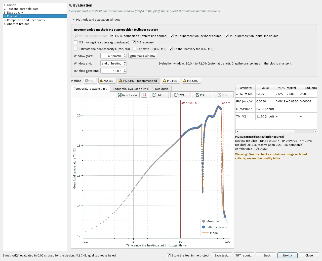
Enter test geometry and undisturbed temperature. Choose ILS, finite-line, cylindrical or short-time fitting models as offered. Inspect screening and fitting start time, power stability, fitted conductivity and resistance, residuals and uncertainty. Early transients and variable heat input can bias a simple line-source fit.
Step-by-step workflows · Menus and keyboard
| Control | Meaning / action | Unit | Range / choices | Example value |
|---|---|---|---|---|
| Methods and evaluation window | Runs the named tool action. | |||
| Reset view | Show all data (also: double-click the plot). | |||
| Chart style button | Chart style: title, axis titles, legend, colours, line widths and markers, fonts, grid and background (also in the chart's context menu). | |||
| PNG… | Export the plot as a PNG image. | |||
| SVG… | Export the plot as a vector SVG image (for Word, Inkscape, …). | |||
| PDF… | Export the plot as a vector PDF. | |||
| CSV… | Export the plotted data as CSV. | |||
| M1 | M1 line-source slope (Mogensen 1983): straight line through Tf against ln t in the evaluation window, Tf = knbsp;lnnbsp;t + m.λ = Q̄ / (4π H k), Rb* = (m − T0)/q̄ − [ln(4α/rb²) − γ] / (4πλ).Needs a constant heating power: drifts and interruptions bias it.The data are unsuitable for this method; this result cannot be selected.Quality checks contain warnings or failed criteria; review the quality table.M1 assumes constant heating power: fluctuations or interruptions make this slope unsuitable; use superposition (M2)M1 conductivity changes by 49.5 % across later fitting starts (screening limit 10.0 %) | |||
| M2 ILS | M2 parameter estimation with temporal superposition of the measured power, forward model: infinite line source (ILS).Tf(t) = T0 + Rb*nbsp;q̃(t) + 1/(2πλ) Σ Δqk G(t − tk), fitted by Levenberg–Marquardt.Robust to power fluctuations and interruptions; 95 % confidence intervals from the parameter covariance. | |||
| M2 CHS – recommended | M2 parameter estimation with temporal superposition of the measured power, forward model: infinite cylinder source (CHS).Tf(t) = T0 + Rb*nbsp;q̃(t) + 1/(2πλ) Σ Δqk G(t − tk), fitted by Levenberg–Marquardt.Robust to power fluctuations and interruptions; 95 % confidence intervals from the parameter covariance. | |||
| M2 FLS | M2 parameter estimation with temporal superposition of the measured power, forward model: finite line source (FLS).Tf(t) = T0 + Rb*nbsp;q̃(t) + 1/(2πλ) Σ Δqk G(t − tk), fitted by Levenberg–Marquardt.Robust to power fluctuations and interruptions; 95 % confidence intervals from the parameter covariance. | |||
| M5 CHS | M5 recovery: the temperature decline after the heating stops, fitted with the whole heating history superposed (kernel of the M2 model); classic form Tf − T0 = Q̄/(4πλH) ln(t/(t − th)).An independent check of λ and T0. | |||
| M1 line-source slope | M1 line-source slope (Mogensen 1983): straight line through Tf against ln t in the evaluation window, Tf = knbsp;lnnbsp;t + m.λ = Q̄ / (4π H k), Rb* = (m − T0)/q̄ − [ln(4α/rb²) − γ] / (4πλ).Needs a constant heating power: drifts and interruptions bias it.The data are unsuitable for this method; this result cannot be selected.Quality checks contain warnings or failed criteria; review the quality table.M1 assumes constant heating power: fluctuations or interruptions make this slope unsuitable; use superposition (M2)M1 conductivity changes by 49.5 % across later fitting starts (screening limit 10.0 %) | |||
| M2 superposition (infinite line source) | M2 parameter estimation with temporal superposition of the measured power, forward model: infinite line source (ILS).Tf(t) = T0 + Rb*nbsp;q̃(t) + 1/(2πλ) Σ Δqk G(t − tk), fitted by Levenberg–Marquardt.Robust to power fluctuations and interruptions; 95 % confidence intervals from the parameter covariance. | |||
| M2 superposition (cylinder source) | M2 parameter estimation with temporal superposition of the measured power, forward model: infinite cylinder source (CHS).Tf(t) = T0 + Rb*nbsp;q̃(t) + 1/(2πλ) Σ Δqk G(t − tk), fitted by Levenberg–Marquardt.Robust to power fluctuations and interruptions; 95 % confidence intervals from the parameter covariance. | |||
| M2 superposition (finite line source) | M2 parameter estimation with temporal superposition of the measured power, forward model: finite line source (FLS).Tf(t) = T0 + Rb*nbsp;q̃(t) + 1/(2πλ) Σ Δqk G(t − tk), fitted by Levenberg–Marquardt.Robust to power fluctuations and interruptions; 95 % confidence intervals from the parameter covariance. | |||
| M3 moving line source (groundwater) | M3 moving line source (groundwater): estimates λ, Rb* and the Darcy velocity u.Identifiable only when vT² t / (4α) ≳ 0.05; the flow direction cannot be found from one borehole. A bounded test domain (sandbox) or a drifting power also look like advection. | |||
| M5 recovery | M5 recovery: the temperature decline after the heating stops, fitted with the whole heating history superposed (kernel of the M2 model); classic form Tf − T0 = Q̄/(4πλH) ln(t/(t − th)).An independent check of λ and T0. | |||
| Estimate the heat capacity C (M2, M3) | C is usually poorly determined by a TRT (strongly correlated with λ) | |||
| Estimate T0 (M2, M3) | Enables or disables this option. | |||
| Fit the recovery too (M2, M3) | The recovery samples after the heating stop are fitted with the same model | |||
| Window start: | Start of the evaluation window since the heating start (automatic: max(10 h, 5 rb²/α)) | h | -0.1 to 10000 | -0.1 |
| Window end: | End of the evaluation window since the heating start | h | -0.1 to 10000 | -0.1 |
| Rb* time constant: | Time constant of the borehole's own response: the Rb* term of M2/M3 follows the power with this lag (heat capacity of fluid and grout; 0 = steady state) | h | 0 to 24 | 1 |
| Automatic window | Choose an automatic fitting window from the screening criteria; inspect it before fitting. | |||
| M1 | M1 line-source slope (Mogensen 1983): straight line through Tf against ln t in the evaluation window, Tf = knbsp;lnnbsp;t + m.λ = Q̄ / (4π H k), Rb* = (m − T0)/q̄ − [ln(4α/rb²) − γ] / (4πλ).Needs a constant heating power: drifts and interruptions bias it.The data are unsuitable for this method; this result cannot be selected.Quality checks contain warnings or failed criteria; review the quality table.M1 assumes constant heating power: fluctuations or interruptions make this slope unsuitable; use superposition (M2)M1 conductivity changes by 15.9 % across later fitting starts (screening limit 10.0 %) | |||
| M2 ILS – recommended | M2 parameter estimation with temporal superposition of the measured power, forward model: infinite line source (ILS).Tf(t) = T0 + Rb*nbsp;q̃(t) + 1/(2πλ) Σ Δqk G(t − tk), fitted by Levenberg–Marquardt.Robust to power fluctuations and interruptions; 95 % confidence intervals from the parameter covariance. | |||
| M2 CHS | M2 parameter estimation with temporal superposition of the measured power, forward model: infinite cylinder source (CHS).Tf(t) = T0 + Rb*nbsp;q̃(t) + 1/(2πλ) Σ Δqk G(t − tk), fitted by Levenberg–Marquardt.Robust to power fluctuations and interruptions; 95 % confidence intervals from the parameter covariance. | |||
| M1 line-source slope | M1 line-source slope (Mogensen 1983): straight line through Tf against ln t in the evaluation window, Tf = knbsp;lnnbsp;t + m.λ = Q̄ / (4π H k), Rb* = (m − T0)/q̄ − [ln(4α/rb²) − γ] / (4πλ).Needs a constant heating power: drifts and interruptions bias it.The data are unsuitable for this method; this result cannot be selected.Quality checks contain warnings or failed criteria; review the quality table.M1 assumes constant heating power: fluctuations or interruptions make this slope unsuitable; use superposition (M2)M1 conductivity changes by 15.9 % across later fitting starts (screening limit 10.0 %) | |||
| M5 recovery | M5 recovery: the temperature decline after the heating stops, fitted with the whole heating history superposed (kernel of the M2 model); classic form Tf − T0 = Q̄/(4πλH) ln(t/(t − th)).An independent check of λ and T0.No recovery phase was recorded; M5 requires measurements after heating stops. |