 BoreTherm
TRT evaluation wizard
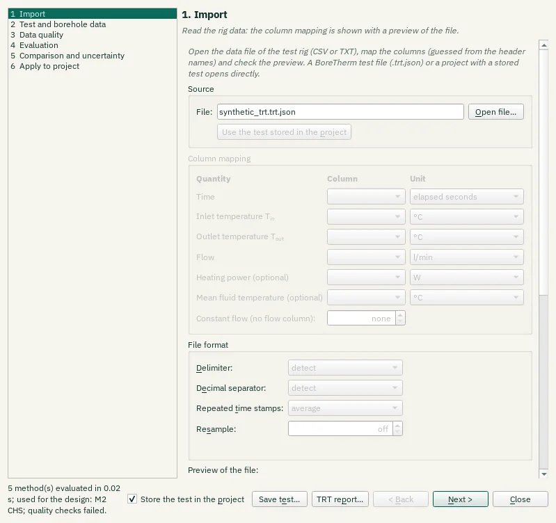
Follow import, test description, screening/evaluation, comparison, report and apply steps. Next and Back navigate without accepting a fit into the design. Apply is explicit; retain the original test data and report for traceability.
Step-by-step workflows · Menus and keyboard
| Control | Meaning / action | Unit | Range / choices | Example value |
|---|---|---|---|---|
| Ground thermal conductivity λ | Enables or disables this option. | |||
| Layer: | λTRT is the effective value over the test borehole's active length. In layered ground it can go to every layer, or to one layer whose value is then chosen so that the effective conductivity over the test length equals λTRT. | Homogeneous ground | ||
| Match the effective value over the test length | Enables or disables this option. | |||
| Volumetric heat capacity C (only when estimated) | Enables or disables this option. | |||
| Mean ground surface temperature, back-computed from T0 | The surface temperature is shifted so that the project's undisturbed temperature over the test length equals T0 of the test (with the project's geothermal heat flux) | |||
| Borehole resistance: | Grout calibration: the grout conductivity is set so that the multipole Rb* of the test borehole at the test flow equals Rb* of the test; Rb* then still follows the design flow and length. Fixed: Rb* is used as it is for every flow and length. | Calibrate the grout conductivity (recommended) / Fixed Rb* / Do not change | ||
| Darcy velocity (M3; stored only) | Enables or disables this option. | |||
| Apply to project | Writes the changes above and the test (data and setup) into the project in one step | |||
| Undo apply | Undo the last TRT-to-design Apply operation. | |||
| Use the values of: | The recommended applicable fit is selected automatically. You can choose another applicable fit; unavailable methods are greyed out and explain why in their tooltips. | Automatic recommendation (M2 CHS) / M1 line-source slope — not applicable / M2 superposition (infinite line source) — Review required / M2 superposition (cylinder source) — Review required (recommended) / M2 superposition (finite line source) — Review required / M3 moving line source (groundwater) — not applicable / M5 recovery (CHS) — Review required | ||
| Back to the automatic choice | Discard your choice: the automatic rule selects the fit again | |||
| Samples: | Realisations of the input errors (0 = off; 200 to 1,000 give stable P5/P95) | 0 to 100000 | 200 | |
| Seed: | Seed of the random numbers: the same seed gives the same result | |||
| Power: | Heating power meter (measured power) | % | 0 to 50 | 2 |
| Flow: | Flow meter (power from flow and ΔT) | % | 0 to 50 | 1 |
| Temperature sensors: | Offset of each temperature sensor | K | 0 to 5 | 0.05 |
| Length H: | Active borehole length | m | 0 to 50 | 0.5 |
| Borehole radius: | Borehole radius | mm | 0 to 50 | 2 |
| Heat capacity C: | Volumetric heat capacity of the ground | % | 0 to 100 | 10 |
| T0: | Undisturbed ground temperature | K | 0 to 10 | 0.2 |
| Run Monte Carlo | Validate the uncertainty setup and start the configured samples. | |||
| Histograms of: | Select one of the listed alternatives. | |||
| Reset view | Show all data (also: double-click the plot). | |||
| Chart style button | Chart style: title, axis titles, legend, colours, line widths and markers, fonts, grid and background (also in the chart's context menu). | |||
| PNG… | Export the plot as a PNG image. | |||
| SVG… | Export the plot as a vector SVG image (for Word, Inkscape, …). | |||
| PDF… | Export the plot as a vector PDF. | |||
| CSV… | Export the plotted data as CSV. | |||
| Methods and evaluation window | Runs the named tool action. | |||
| M1 | M1 line-source slope (Mogensen 1983): straight line through Tf against ln t in the evaluation window, Tf = knbsp;lnnbsp;t + m.λ = Q̄ / (4π H k), Rb* = (m − T0)/q̄ − [ln(4α/rb²) − γ] / (4πλ).Needs a constant heating power: drifts and interruptions bias it.The data are unsuitable for this method; this result cannot be selected.Quality checks contain warnings or failed criteria; review the quality table.M1 assumes constant heating power: fluctuations or interruptions make this slope unsuitable; use superposition (M2)M1 conductivity changes by 49.5 % across later fitting starts (screening limit 10.0 %) | |||
| M2 ILS | M2 parameter estimation with temporal superposition of the measured power, forward model: infinite line source (ILS).Tf(t) = T0 + Rb*nbsp;q̃(t) + 1/(2πλ) Σ Δqk G(t − tk), fitted by Levenberg–Marquardt.Robust to power fluctuations and interruptions; 95 % confidence intervals from the parameter covariance. | |||
| M2 CHS – recommended | M2 parameter estimation with temporal superposition of the measured power, forward model: infinite cylinder source (CHS).Tf(t) = T0 + Rb*nbsp;q̃(t) + 1/(2πλ) Σ Δqk G(t − tk), fitted by Levenberg–Marquardt.Robust to power fluctuations and interruptions; 95 % confidence intervals from the parameter covariance. | |||
| M2 FLS | M2 parameter estimation with temporal superposition of the measured power, forward model: finite line source (FLS).Tf(t) = T0 + Rb*nbsp;q̃(t) + 1/(2πλ) Σ Δqk G(t − tk), fitted by Levenberg–Marquardt.Robust to power fluctuations and interruptions; 95 % confidence intervals from the parameter covariance. | |||
| M5 CHS | M5 recovery: the temperature decline after the heating stops, fitted with the whole heating history superposed (kernel of the M2 model); classic form Tf − T0 = Q̄/(4πλH) ln(t/(t − th)).An independent check of λ and T0. | |||
| M1 line-source slope | M1 line-source slope (Mogensen 1983): straight line through Tf against ln t in the evaluation window, Tf = knbsp;lnnbsp;t + m.λ = Q̄ / (4π H k), Rb* = (m − T0)/q̄ − [ln(4α/rb²) − γ] / (4πλ).Needs a constant heating power: drifts and interruptions bias it.The data are unsuitable for this method; this result cannot be selected.Quality checks contain warnings or failed criteria; review the quality table.M1 assumes constant heating power: fluctuations or interruptions make this slope unsuitable; use superposition (M2)M1 conductivity changes by 49.5 % across later fitting starts (screening limit 10.0 %) | |||
| M2 superposition (infinite line source) | M2 parameter estimation with temporal superposition of the measured power, forward model: infinite line source (ILS).Tf(t) = T0 + Rb*nbsp;q̃(t) + 1/(2πλ) Σ Δqk G(t − tk), fitted by Levenberg–Marquardt.Robust to power fluctuations and interruptions; 95 % confidence intervals from the parameter covariance. | |||
| M2 superposition (cylinder source) | M2 parameter estimation with temporal superposition of the measured power, forward model: infinite cylinder source (CHS).Tf(t) = T0 + Rb*nbsp;q̃(t) + 1/(2πλ) Σ Δqk G(t − tk), fitted by Levenberg–Marquardt.Robust to power fluctuations and interruptions; 95 % confidence intervals from the parameter covariance. | |||
| M2 superposition (finite line source) | M2 parameter estimation with temporal superposition of the measured power, forward model: finite line source (FLS).Tf(t) = T0 + Rb*nbsp;q̃(t) + 1/(2πλ) Σ Δqk G(t − tk), fitted by Levenberg–Marquardt.Robust to power fluctuations and interruptions; 95 % confidence intervals from the parameter covariance. | |||
| M3 moving line source (groundwater) | M3 moving line source (groundwater): estimates λ, Rb* and the Darcy velocity u.Identifiable only when vT² t / (4α) ≳ 0.05; the flow direction cannot be found from one borehole. A bounded test domain (sandbox) or a drifting power also look like advection. | |||
| M5 recovery | M5 recovery: the temperature decline after the heating stops, fitted with the whole heating history superposed (kernel of the M2 model); classic form Tf − T0 = Q̄/(4πλH) ln(t/(t − th)).An independent check of λ and T0. | |||
| Estimate the heat capacity C (M2, M3) | C is usually poorly determined by a TRT (strongly correlated with λ) | |||
| Estimate T0 (M2, M3) | Enables or disables this option. | |||
| Fit the recovery too (M2, M3) | The recovery samples after the heating stop are fitted with the same model | |||
| Window start: | Start of the evaluation window since the heating start (automatic: max(10 h, 5 rb²/α)) | h | -0.1 to 10000 | -0.1 |
| Window end: | End of the evaluation window since the heating start | h | -0.1 to 10000 | -0.1 |
| Rb* time constant: | Time constant of the borehole's own response: the Rb* term of M2/M3 follows the power with this lag (heat capacity of fluid and grout; 0 = steady state) | h | 0 to 24 | 1 |
| Automatic window | Choose an automatic fitting window from the screening criteria; inspect it before fitting. | |||
| Drag to exclude an interval | On: a drag across a plot excludes that interval. Off: a drag moves the view. | |||
| Automatically exclude suspect readings | Exclude detected temperature outliers and flow/power disturbances from fitting. Raw readings and measured heat history are preserved. | |||
| Interval time unit | Unit used for the start and end of excluded observation intervals. | Hours since heating start / Seconds in the data | ||
| From | Enter a numerical value in the shown units. | -1e+12 to 1e+12 | 0 | |
| To | Enter a numerical value in the shown units. | -1e+12 to 1e+12 | 0 | |
| Add interval | Add an observation-exclusion interval with start/end times. | |||
| Remove | Remove the selected evaluation item or interval from this table. | |||
| Clear all | Remove the manually selected exclusion intervals. | |||
| Copy borehole, pipes, fluid and ground from the project | Copy the design construction and material settings into this TRT setup; confirm they describe the measured test. | |||
| Length H: | Active length of the test borehole | m | 1 to 3000 | 150 |
| Buried depth D: | Depth of the top of the active length | m | 0 to 500 | 2 |
| Borehole diameter: | Borehole diameter (2 rb) | mm | 50 to 600 | 152 |
| Time since grouting: | Days between grouting and the start of the test (quality check) | days | -1 to 3650 | 7 |
| Pipe type: | Select one of the listed alternatives. | Single-U / Double-U / Triple-U / Coaxial / Multi-U (4–8) / Helix (spiral coil) | ||
| Pipe outer diameter: | Outer diameter of the pipes (coaxial: outer pipe) | mm | 10 to 200 | 40 |
| Pipe wall thickness: | Wall thickness of the pipes | mm | 0.5 to 20 | 3.7 |
| Shank spacing: | Centre-to-centre distance of opposite legs | mm | 0 to 300 | 85 |
| Grout conductivity: | Thermal conductivity of the grout | W/(m·K) | 0.1 to 10 | 2 |
| Pipe conductivity: | Thermal conductivity of the pipe wall | W/(m·K) | 0.05 to 60 | 0.42 |
| Fluid: | Select one of the listed alternatives. | Water / / Glycols / Monoethylene glycol (MEG) / Monopropylene glycol (MPG) / / Alcohols / Ethanol / Methanol / / Salt solutions / Potassium formate / Potassium acetate / Potassium carbonate / Calcium chloride / Sodium chloride / / Glycerol / / Custom (constant properties) / Table (temperature-dependent) | ||
| Mass fraction: | Mass fraction of the antifreeze | % | 0 to 60 | 0 |
| Heat capacity C: | Volumetric heat capacity of the ground: fixed in the evaluation unless it is estimated | MJ/(m³·K) | 0.5 to 5 | 2.2 |
| Surface temperature: | Mean ground surface temperature (T0 plausibility check) | °C | -20.1 to 40 | 9.5 |
| Geothermal heat flux: | Geothermal heat flux (T0 plausibility check) | W/m² | -0.005 to 0.3 | 0.065 |
| Method: | Select one of the listed alternatives. | Initial circulation (before the heating) / Manual value / Depth profile (mean over the active length) | ||
| Averaging window: | Averaging window before the heating start | min | 1 to 1440 | 60 |
| T0 (manual): | Undisturbed ground temperature | °C | -10.1 to 100 | -10.1 |
| Add depth | Add a depth-resolved TRT input row. | |||
| Remove depth | Remove the selected depth-resolved input row. | |||
| Power: | Q = ρ cp V̇ (Tin − Tout) with the fluid properties at the mean fluid temperature, or the heater / heat meter column | Measured (power column) / From flow and ΔT (inlet − outlet) | ||
| Heating start: | Start of the heating in the time of the data | h | -1000 to 10000 | 1 |
| Heating end: | End of the heating since its start; the recovery follows (automatic: the last sample with heating power) | h | -0.1 to 10000 | -0.1 |
| Selected test file | The local test data file selected for import. | |||
| Open file… | Rig data (CSV, TXT, DAT), a BoreTherm test file (.trt.json) or a project with a stored test | |||
| Use the test stored in the project | Load the TRT data already embedded in the open project. | |||
| Time column | Map the source column for this quantity. Leave not mapped only when the required quantity can be supplied by another supported input. | |||
| Time unit | Select the source unit before import. | elapsed seconds / elapsed minutes / elapsed hours / elapsed days / date and time (detected) / dd.mm.yyyy HH:MM / dd.mm.yyyy HH:MM:SS / mm/dd/yyyy HH:MM:SS | ||
| Inlet temperature column | Map the source column for this quantity. Leave not mapped only when the required quantity can be supplied by another supported input. | |||
| Inlet temperature unit | Select the source unit before import. | °C / K / °F | ||
| Outlet temperature column | Map the source column for this quantity. Leave not mapped only when the required quantity can be supplied by another supported input. | |||
| Outlet temperature unit | Select the source unit before import. | °C / K / °F | ||
| Flow column | Map the source column for this quantity. Leave not mapped only when the required quantity can be supplied by another supported input. | |||
| Flow unit | Select the source unit before import. | l/min / l/s / l/h / m³/h / m³/s / kg/s | ||
| Heat input column | Map the source column for this quantity. Leave not mapped only when the required quantity can be supplied by another supported input. | |||
| Heat input unit | Select the source unit before import. | W / kW / MW | ||
| Mean temperature column | Map the source column for this quantity. Leave not mapped only when the required quantity can be supplied by another supported input. | |||
| Mean temperature unit | Select the source unit before import. | °C / K / °F | ||
| Trt constant flow | Constant flow of the test when the file has no flow column (0 = none) | l/min | 0 to 10000 | 0 |
| Delimiter: | Select one of the listed alternatives. | detect / semicolon ; / comma , / tab / spaces | ||
| Decimal separator: | Select one of the listed alternatives. | detect / point 1.5 / comma 1,5 | ||
| Repeated time stamps: | Samples with the same time stamp, e.g. 30 s data with minute stamps | average / spread to the next stamp / keep | ||
| Resample: | Averages the samples on a uniform time step (0 = keep every sample) | s | 0 to 3600 | 0 |
| Fibre position of the ground surface: depth = position - offset | Fibre position of the ground surface: depth = position - offset | m | -10000 to 10000 | 0 |
| Top of the depth range of the mean | Top of the depth range of the mean | m | -10000 to 10000 | 0 |
| Bottom of the depth range of the mean (e.g. the borehole length) | Bottom of the depth range of the mean (e.g. the borehole length) | m | -10000 to 10000 | 100 |
| Added to the DTS times after the calendar times are matched (e.g. -1 h for a DTS in UTC and a logger in CET) | Added to the DTS times after the calendar times are matched (e.g. -1 h for a DTS in UTC and a logger in CET) | h | -48 to 48 | 0 |
| Depth mean as the mean fluid temperature | The mean over the depth range of every DTS profile becomes the mean fluid temperature of the records (one-minute values). | |||
| Add DTS file… | Links a DTS file (fibre position in the first column, one column per time stamp) to the test | |||
| Read the full data | Reads the full data of the compact copy again from the linked files | |||
| Store the test in the project | On closing, the records and the evaluation setup are kept in the project file (the report uses them); the design values change only with Apply. | |||
| Save test… | Save the records and the setup as a BoreTherm test file (.trt.json), e.g. for boretherm-cli trt | |||
| TRT report… | Write the TRT evaluation report (VDI 4640 Part 5 contents) as PDF or HTML | |||
| < Back | Return to the previous wizard step. | |||
| Next > | Continue to the next wizard step. | |||
| Close | Close this view. | |||
| Histograms of: | Select one of the listed alternatives. | M1 line-source slope / M2 superposition (cylinder source) |