The steady model of Chapters 5 and 8 treats the inside of the borehole as a resistance: at every time. The fluid, the pipes and the grout store no heat, so a load step reaches the fluid temperature at once and in full. The borehole model is an option:
| Model | What it adds | Status |
|---|---|---|
| Steady resistance (default) | nothing; the model of the classic monthly method | the classical results |
| Short-time capacity | the heat capacity of fluid, pipes and grout at short times, as a combined response | available |
| Dynamic | transient fluid and grout along the depth, transit delay, flow schedule (TRCM network) | a separate transient model, not treated here |
The classic monthly method has neither of the new models; the classic-method preset resets the model to the steady resistance.
15.1 Equivalent single pipe
The legs of a U-tube borehole ( = 2, 4, 6) are replaced by one concentric pipe (Xu & Spitler 2006) that keeps the fluid volume and the pipe-wall volume (, ), the film and wall resistances of the pipes in parallel, and the effective borehole resistance: the grout annulus gets the conductivity that makes
Xu & Spitler keep ; keeping makes the long-time end of the model equal to the steady model, including the short-circuit term, and lets the correction start at 0. Coaxial: the outer pipe is already concentric, and the whole fluid is one well-mixed node (the inner channel's capacity is slightly overstated). Sections enter as length-weighted equivalents (mean radius, sectioned , mean grout capacity). Heat capacities: fluid at the property temperature, pipe walls 1.8 MJ/(m³ K), grout as given in the borehole design (default 2.0 MJ/(m³ K)), ground of the ground reference.
15.2 Radial model and the combined response
A one-dimensional radial finite-volume model (a well-mixed fluid node, 3 pipe-wall cells, 12 grout cells and 90 log-spaced ground cells out to ) receives a unit step heat rate in the fluid node and is integrated with variable-step BDF2 (about 320 steps to 100 h). It is run twice, with and without the capacities of fluid, pipes and grout; the difference is the capacity correction
with a blend weight for and a smoothstep in to 0 at = 100 h. starts near (the fluid has not warmed yet) and tends to 0; at 100 h the unblended capacity effect is below 0.3 % of the response. The combined response
is tabulated at 40 nodes per decade from 1 min to and interpolated in ; below 1 min it is linear in from 0, from on it is exactly . In the first minutes the radial wall warms faster than the line-source , so the table is kept , non-decreasing and . With all capacities 0 the correction is exactly 0. Two radial runs take under 1 ms and are repeated at every simulation and sizing iteration ( depends on H).
15.3 Use in the simulation
Everything the steady model computes stays; the capacity correction is added as a short convolution:
with = 1 h and fewer than 100 terms, the same for the FFT and the load-aggregation method, so the steady part is untouched. The monthly base temperatures are unchanged (the correction is 0 after 100 h); the peak pulses of (8.4) use , also with the classic asymptote (8.5).
| Example | steady → short-time [°C] | steady → short-time [°C] | max hourly | Sized H [m] |
|---|---|---|---|---|
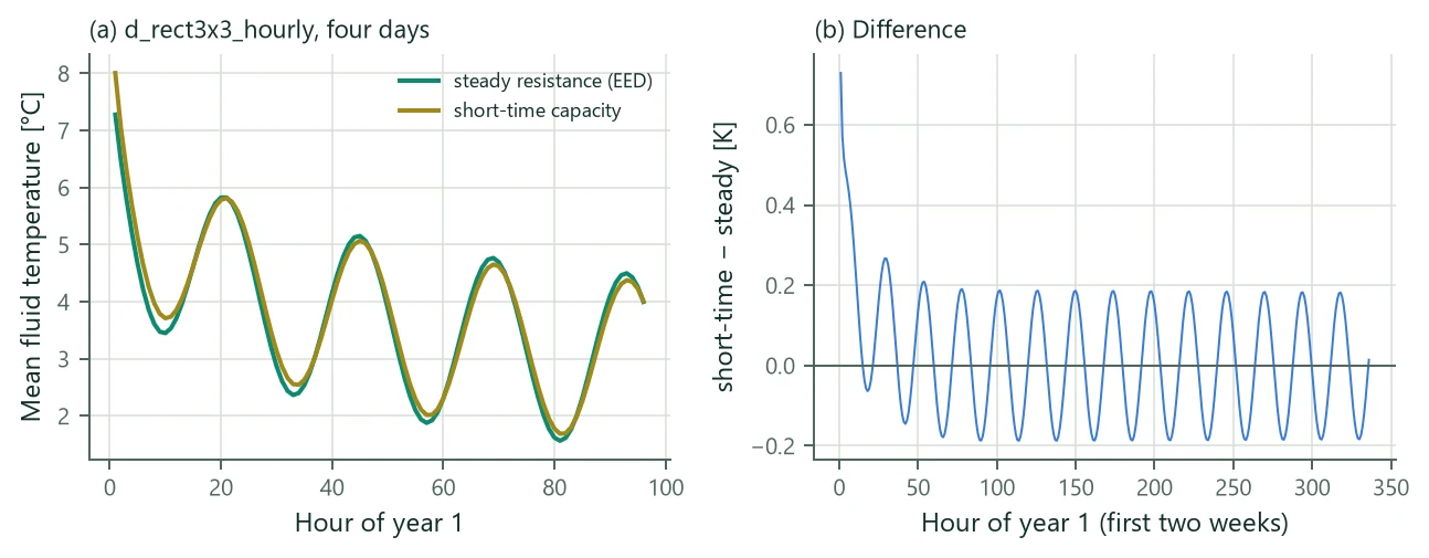
| 3 × 3 field, hourly loads | −0.130 → −0.010 | 22.416 → 22.288 | 0.73 K | – |
| Sizing case, hourly | −4.342 → −4.170 | 21.883 → 21.742 | 1.00 K | 117.26 → 116.02 |
| Office example (4 × 4) | −2.413 → −2.244 | 16.026 → 15.925 | – | 143.72 → 141.89 |
| Sizing case, monthly | −5.098 → −4.943 | 22.524 → 22.397 | – | 122.70 → 121.59 |
| Linden worked example | −15.575 → −15.299 | 21.438 → 21.001 | – | – |
| Ahmadfard & Bernier (2019), case 3, 6 h peaks | −2.084 → −1.803 | 29.072 → 28.691 | – | 110.93 → 108.34 |
Short peaks of a few hours are 0.1–0.45 K less extreme and sizing is 1–2.5 % shorter where they bind; hourly moves by up to 1 K in the first hours after a load change (Figure 13). A single borehole with 10 kW monthly peaks of 2 h needs 219.0 m with the steady model and 210.4 m with the short-time model.
15.4 TRCM parameters from the multipole matrix
Transient borehole models (a dynamic model along the depth, a finite-element borehole element) use the thermal resistance and capacity model (TRCM) of Bauer et al. (2011): every leg has a fluid node and a grout node ; is connected to through , to the borehole wall through , and the grout nodes to each other through , with
Bauer et al. give and the grout–grout resistance from two-pipe line-source formulas. BoreTherm derives them from the multipole matrix of Chapter 5 (with sleeves and casing) so that the steady network reproduces it exactly. With , , and the grout Laplacian , eliminating the grout nodes gives , hence
For a single U-tube this is Bauer's with his grout–grout resistance. The grout-node position is Bauer's
( the borehole and the pipe diameter; = 2 and 4 are Bauer's single- and double-U formulas, triple-U uses 6). Second law: and must be positive definite and ; otherwise (Diersch et al. 2011). The steady TRCM discretised along the depth at a uniform wall temperature reproduces Hellström's leg temperatures and (5.22).
15.5 Incremental load aggregation
The Claesson–Javed cells of (8.10)–(8.11) are also available one step at a time for time-stepping models and co-simulation, with four operations: commit a step with its load; the value, the response at the end of the last committed step (the batch computation is a loop over commit and value and bit-identical to the incremental result); the history, the response at the end of the next step to the committed loads only; and the partial step with and , the response a fraction into the next step with the running mean load of its elapsed part:
with the cells as the next commit would shift them; the partial step with load and equals the value after committing exactly. Every commit conserves the energy of the loads, and the state can be saved and restored (rollback of a co-simulation step).