Most projects start from monthly loads: the heating, cooling and domestic hot water (DHW) energy of every month and a peak power with its duration. The classic monthly method works with exactly these values. Hourly loads put the daily cycle into the design, and the dynamic borehole model needs them, but measured or simulated hourly loads are often not available in early design. Two tools of the Loads page close these gaps: the hourly load generator, which turns the monthly table into a synthetic hourly profile, and monthly loads per year, which give every operating year its own monthly table, entered directly, imported, or built with the load growth helper. All loads in this chapter are building loads in kW or MWh; their conversion to ground loads with the seasonal performance factors is the same as for any other load input.
25.1 Months and hours
The generator works with the 730-hour months that the monthly simulation uses: hour () is hour of operating month . Month belongs to operating year (rounded down) and to calendar month counted modulo 12, with the start month of the simulation, so hour 0 is the first hour of the start month, as in the hourly simulation. One year of 8760 hours is generated (the simulation repeats it), or years when the monthly loads per year are switched on.
25.2 Synthetic outdoor temperature
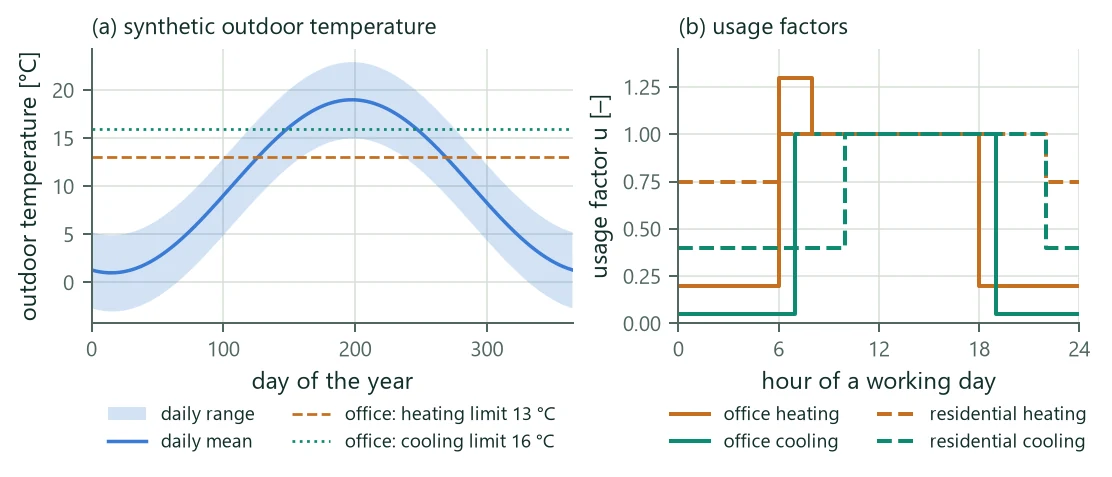
The hours of a month are weighted by an outdoor temperature (the degree-hour approach) and a use pattern. The outdoor temperature is synthetic: with the day of the year and the hour of the day,
with the annual mean , the annual amplitude (half the difference between the smooth warmest and coldest day), the coldest day and the daily amplitude (warmest at 15 h). The weather term is a daily anomaly that follows a first-order autoregressive process,
with the stationary standard deviation (the weather variation), interpolated linearly between the middles of the days so that the temperature has no jumps at midnight. The numbers are standard normal deviates by the Box–Muller method (Box and Muller 1958) from a fully specified random number generator, so the profile is the same for the same seed. The defaults describe central Europe: = 10 °C, = 9 K, = 4 K, = 3 K, = 15 (15 January). The temperature is not a weather record of a site; it only orders the hours of a month by their likely demand.
25.3 Weights and use patterns
Every hour gets a weight per load column:
and are the heating and cooling limits of the degree-hours, and is the degree-hour offset (default 1 K): loads also occur in hours without degree-hours, through internal gains, losses and hot-water circulation, and the offset keeps those hours from receiving nothing. The usage factors of the pattern depend on the hour and on the day of the week, which follows from the weekday of 1 January and the start of operation (Table 49, Figure 22). The equal method gives every hour the weight 1 and does not use a pattern.
| Pattern | Heating | Cooling | DHW | / |
|---|---|---|---|---|
| Residential | 1 from 6 to 22 h, 0.75 at night (set-back) | 1 from 10 to 22 h, 0.4 otherwise | daily draw-off profile with peaks at 7 h (2.2) and 19 h (1.8), mean 1 | 15 / 20 °C |
| Office | working days 6–18 h: 1 (6–8 h: 1.3, morning boost), otherwise 0.2 | working days 7–19 h: 1, otherwise 0.05 | working days 7–18 h: 1, otherwise 0.05 | 13 / 16 °C (internal gains) |
| Continuous | 1 | 1 | 1 | 15 / 18 °C |
25.4 Distribution with an upper limit
The month's energy is distributed over its hours with the weights and an upper limit on every hour ("water filling"):
is found by sorting the weights: the largest hours sit at , and with the smallest for which the next hour stays below . Without a limit . Hours of zero weight receive energy only when the weighted hours cannot hold below ; all-zero weights count as equal. The distribution requires , and the sum of the hours equals to rounding (relative ).
25.5 Peaks
The monthly table gives a peak power with a duration for heating and cooling. With peaks switched on and both positive, the peak takes = max(1, round()) hours:
- h (the peak is not above the month's mean power): the peak is not used and the energy is spread by the weights alone (with a note).
- h (less than one hour at the peak power): the peak cannot be reached, and the energy is distributed below by (25.4) (with a note).
- Otherwise is limited to the number of whole hours the energy can hold at (a note when it shrinks). A peak block of consecutive hours is set to , and the rest is spread over the other hours by (25.4) with as the limit. The block lies either at the consecutive hours with the largest sum of weights (the coldest hours for heating, the warmest for cooling; with equal weights the end of the month) or at the end of the month, where the monthly model places its peak pulse. The month keeps its energy exactly and its largest hour is ; more than hours can reach when the pattern concentrates the demand.
A second rule follows the classic monthly method, which adds the peak on top of the mean load: the hours get and the block hours become , so the month's energy grows by the peak energy. With the equal method and the block at the month end this reproduces the hourly loads that the classic method derives from monthly loads, and the hourly simulation then gives the annual extremes of the monthly model within 0.08 K for the verification example. DHW has no peak in the monthly table and is spread by its weights; the heating peak applies to the heating column alone, as in the monthly model.
25.6 Example: an office building
The generator reports, per year and load column, the energy, the largest hour and the full-load hours , and compares the month energies of the table with the generated ones. Table 50 gives them for an office building with 200 MWh of space heating, 45 MWh of cooling and 8 MWh of DHW a year, generated with the office pattern (8760 hours).
| Column | Energy [MWh/a] | Largest hour [kW] | Full-load hours [h] |
|---|---|---|---|
| Heating | 200.0 | 100.0 | 2000 |
| Cooling | 45.0 | 45.0 | 1000 |
| DHW | 8.0 | 2.7 | 2946 |
The energies equal those of the monthly table, and the largest heating hour is the heating peak power of the table (100 kW). The design consequence is substantial. The office draws its peak for a whole working day, day after day, while the monthly model assumes 6 hours at the end of a month at mean load. On a field of 16 boreholes of 150 m over 25 years the lowest hourly mean fluid temperature is −3.06 °C against −2.41 °C with the monthly model, and Size borehole length gives 150.7 m with the hourly loads against 143.7 m with the monthly loads (7.0 m per borehole, 112 m for the field, at a lower limit of −3.00 °C). Generated hourly loads keep the monthly energies and peaks, not the real weather; they are assumptions and should be replaced by measured or simulated design loads when those exist.
25.7 Monthly loads per year
Monthly loads per year are an option of the monthly load input, not a separate load mode: the input stays monthly with peaks, so everything that distinguishes monthly from hourly loads keeps working, and the table can be switched off without losing it. Operating year (counted from the start month) uses the table of year , or the last year of the table when the table is shorter, with a warning naming the years that repeat it; a longer table is cut at the design period. With a start month other than January an operating year takes the calendar months and of its row.
The monthly simulation then uses the base load, the peak powers and the peak durations of year and calendar month in the superposition of the monthly method, which is linear in the loads and therefore unchanged; the time grid of the g-function starts at the shortest peak of all years. Without the option every year uses the same table and every result is identical to the single-table calculation. The hourly simulation does not use the option directly; the generator turns the per-year table into years of hourly loads. Sizing, the network results at the temperature extremes and the pre-conditioning of the co-simulation use the year-specific loads too.
Tables per year can be exported and imported as text files with one row per year and month (heating, cooling and DHW energy, heating and cooling peak power with duration). A written table reads back identically; on import, separators, decimal commas, rows in any order and a missing header are accepted, missing months count as zero, and duplicate rows or years outside 1 to 100 are refused.
25.8 Load growth
The load growth helper builds the per-year table from the monthly table as the base. Year (counted from 1) gets the factor
for and before, with the first changed year (default 2: year 1 is the base). The factor is clamped at , so a decline stops at zero. It is applied to the selected energies (heating, cooling, DHW) and optionally to the heating and cooling peak powers with their energy; the peak durations stay. Typical uses are a building that is occupied in stages (linear or compound growth), an extension of the building in a given year (step), and a declining heating demand after a refurbishment (negative ).