A borehole field never sees the building. It sees what the heat pump takes from the ground and puts back. This chapter describes how BoreTherm converts the building loads of a project (space heating, domestic hot water and cooling) into ground loads, with fixed seasonal performance factors or with a heat pump whose performance depends on the fluid temperature of the field, and how the program derives the requirements a brine/water heat pump must meet for a designed field and checks candidate machines against them.
The example used throughout is an office building with monthly loads of 200 MWh/a space heating, 8 MWh/a domestic hot water (DHW) and 45 MWh/a active cooling (peaks 100 kW heating, 45 kW cooling) on a 4 × 4 field of 16 boreholes of 150 m, simulated over 25 years, with a 25 % monopropylene glycol and the mean-fluid-temperature limits −3 °C and +20 °C. Its three candidate heat pumps are fictitious datasheets and are called machine A, B and C here.
27.1 Energy balance of the heat pump
The heat pump delivers the useful heat from the ground heat and the electricity of its compressor. With the coefficient of performance at one operating point, and the energy efficiency ratio in cooling,
In heating the electricity reduces what the ground must deliver; in active cooling the compressor heat is added to what the ground must absorb; passive (free) cooling sends the cooling energy to the ground unchanged, apart from the circulation pump. Over a season the COP becomes the seasonal performance factor SPF, the heat delivered divided by the electricity used. In BoreTherm the SPF always includes the electric backup heater and the source (brine) pump, so it is a system figure and not the rated efficiency of the machine.
27.2 Fixed seasonal performance factors
The quick and transparent method multiplies each building load by a constant ground factor. With the seasonal performance factors (space heating), (hot water) and (active cooling):
- The same factors apply to the peak powers of each month, so a 17 kW heating peak at SPF 2.12 on 200 m of borehole becomes = 44.91 W/m of extraction.
- Monthly energies become mean powers with months of 730 h: per metre of the total borehole length . With monthly loads an annual DHW energy is spread equally over the twelve months.
- and must be greater than 1 (SPF = 1 means no ground extraction; such loads are entered as ground loads directly). A very large makes active cooling effectively direct.
The weakness of the method is that the SPF is an assumption: it does not react when the field becomes colder or warmer over the years, and it is not tied to a machine.
27.3 Temperature-dependent performance
In the temperature-dependent mode the heat pump model gives the COP at every operating point from the actual source and sink temperatures, the borefield is simulated with the ground loads that follow, and the two are iterated until they agree. The SPF is then a result; the SPFs entered for the fixed mode are only the starting values of the first pass. The mode is chosen on the Heat pump › Setup page, which is the only place that decides how the heat pump enters the borefield calculation.
27.3.1 Operating point
The source temperature is that of the brine leaving the field and entering the evaporator. With monthly results it follows from the mean fluid temperature (the mean of inlet and outlet), the heat rate (positive for injection into the ground) and the capacity rate of the field flow; with hourly results the simulated outlet temperature is used directly:
During extraction the outlet is warmer than the mean fluid temperature, so using itself would understate the COP. The sink temperature is the flow temperature of the heating curve, linear between the return temperature at the heating limit and the design flow temperature at the design outdoor temperature and constant outside that range:
Domestic hot water has its own sink temperature (50 °C in the example). The outdoor temperature of each month or hour comes from a seeded synthetic climate (a seasonal cosine around the annual mean, a daily cycle and an autocorrelated day-to-day weather), not from measured weather.
27.3.2 COP models
Temperatures in the Carnot terms are in kelvin; is the temperature difference across the two heat exchangers (5 K by default). Four models are available:
- Datasheet interpolation. Each EN 14511 test point (brine inlet, water outlet, COP, heat output) is divided by its Carnot COP to give an exergetic efficiency . At the operating point, is interpolated linearly in the triangle of test points that contains it, or along the nearest segment (clamped to its end points) outside their convex hull, and multiplied by the local Carnot COP:
Outside the test points the model therefore extrapolates with a constant share of the Carnot COP. The heat output is interpolated in the same way and held at the nearest segment outside the points.
- Carnot efficiency. A constant times the Carnot term of (27.6); with exactly one test point, follows from it.
- Carnot model with load-dependent approaches (the Carnot heat pump with condenser temperature control of Wetter et al. 2014, steady state). It works with the leaving temperatures and approach temperatures that grow with the part-load ratio :
with , and the part-load efficiency with . COP and evaporator outlet depend on each other and are solved by fixed-point iteration; the lift in the denominator is limited smoothly to at least 1 K. The approaches default to 2 K and the nominal point to 35 °C / −3 °C (B0/W35 with a 3 K brine spread). A fixed-speed machine runs at its available capacity while on, so is its capacity over the nominal one; a variable-speed machine follows the load.
- Generic regression. A quadratic in the temperature lift (in K) with a field derating of 0.85; for a brine source , for an air source .
All models give at least COP 1. The default test points of a new project are generic assumptions, not the certified data of a product; they are meant to be replaced by the datasheet of the selected machine.
27.3.3 Ground loads and the coupling loop
In every month (or hour) the heat pump covers the share of the heat it can deliver. Load above its capacity, and all load while the brine is below the minimum source temperature of the machine, goes to an electric backup heater at COP 1, which takes nothing from the ground. The ground factors of the month are
Passive cooling is used only while the field outlet stays at or below the passive cooling limit (16 °C by default; monthly loads check the peak injection case); above it the machine cools actively with its EER. The loop is:
- Pass 1 converts the loads with the SPFs entered for the fixed mode.
- The borefield is simulated over all years, giving and, with (27.4), the source temperature of every month.
- The heat pump model gives the COP at the source temperature and the heating-curve or DHW sink of that month; capacity and minimum source temperature give the backup share.
- New ground factors (27.8) give new ground loads.
- The loop stops when the energy-weighted SPF (and the monthly factors) change by less than 0.01, at most after five passes; a loop that has not converged gives a warning.
One pass is one complete borefield simulation. Sizing (Size borehole length) runs this loop at every trial length, so the sized length and the heat pump are consistent.
27.3.4 Seasonal performance factor and the JAZ after VDI 4650
The simulated SPF divides the delivered heat by all the electricity of heating: compressor, backup heater and source pump; the cooling SEER divides the cold by the cooling electricity including the pump:
With a large field pump the SEER can be far below the EER of the machine: in the sized example the SEER is 2.84 with a machine EER of 5.6. Beside the simulated SPF BoreTherm reports the tabulated annual performance factor (JAZ) of VDI 4650 Blatt 1:2024. For brine/water space heating
with for the operating spread of the heating system against the test spread, over the minimum brine inlet temperature and the maximum supply temperature (separate tables for fixed-speed and variable-capacity machines), the simulated source-pump power and the drive power of the heat pump. Hot water by the heating heat pump gets its own , and the overall value combines both with the hot-water share and the coverage of the heat pump:
For the borefield, is the lowest heat pump inlet (field outlet) temperature of the simulated design: the lowest 168 h mean with hourly loads, the lowest monthly mean with monthly loads (the guideline suggests a weekly mean, which is noted). Intermediate table values are interpolated linearly. The guideline does not allow extrapolation: a supply below 30 °C, hot water below 50 °C or above 5 °C use the conservative table edge; beyond the other edges ( below −3 °C, supply above 60 °C, spreads outside 3–10 K) the JAZ is reported as not applicable. The implementation reproduces the worked examples 8.1 (JAZ 4.75) and 8.3 (3.88) of the guideline.
27.4 Why the COP matters twice
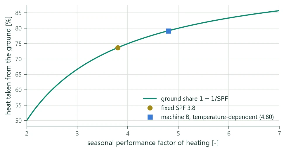
A better heat pump uses less electricity, so a larger share of the heat comes from the ground (Figure 23). A field sized with a pessimistic fixed SPF can therefore be too short for a good machine. Table 54 shows the effect in the example: with the temperature-dependent model of machine B the net ground extraction rises, the lowest mean fluid temperature falls below the −3 °C limit, and the boreholes must be longer. The effect limits itself: a colder field lowers the COP and with it the share from the ground, and the coupling loop finds the balance.
| State | SPF heating | Net ground extraction [MWh/a] | [°C] | Limit −3 °C |
|---|---|---|---|---|
| Fixed SPF 3.8 / 2.8 / 5.0, 150 m | 3.8 (input) | 143.1 | −2.41 | within the limit |
| Machine B as the project's heat pump, 150 m | 4.80 (result) | 160.5 (+12 %) | −3.84 | below the limit |
| Machine B, sized to 160.0 m | 4.82 (result) | 161.1 | −3.00 | at the limit |
27.5 Heat pump selection: purpose and limits
Once a field is designed, the next step is a brine/water heat pump that fits it. BoreTherm gives two things on the Heat pump › Equipment selection and Selection results pages:
- A requirement sheet: what the heat pump must deliver and tolerate for this field (capacity at the design point, evaporator capacity, source and sink temperatures, brine flow and pump head, part-load profile, cooling, seasonal performance). Every line has a value, a unit, how it was obtained, and a flag when the project itself is inconsistent. The sheet needs no candidate.
- A candidate check: candidate machines entered from their datasheets are checked line by line, and the design is simulated again with each candidate in the temperature-dependent mode (the coupled rerun).
It is a preliminary selection. There is no product database; the datasheets are typed in or imported. The engineer must still check the manufacturer's data, the operating envelope, the hydraulics and the controls. No funding threshold, refrigerant, sound or electrical requirement is checked. Editing the selection inputs never changes the design results; only Use in the project (which copies a candidate into the project's heat pump model and switches the mode to temperature-dependent) does, as one undo step, without changing the borehole length.
27.6 Design point
| Definition | Why | |
|---|---|---|
| Outdoor | Monovalent: the design outdoor temperature of the heating curve. Mono-energetic (heat pump with a heating rod): the bivalence temperature. | The heat pump alone must meet the load down to this temperature. |
| Sink | Flow temperature of the heating curve (27.5) at that outdoor temperature. | EN 14511 rates the water outlet (the W of B0/W35). |
| Source | Lowest field outlet temperature with flow over the whole period (monthly: base and peak cases with (27.4); hourly: the hourly outlet). | The field outlet is the evaporator inlet, the B of B0/W35, and is warmer than the mean fluid temperature in heating. |
B0/W35 is the catalogue rating point, not the design point; it is reported for catalogue comparison. The source limits use the mean fluid temperature, which is the more conservative quantity.
27.7 Capacity, evaporator and source limits
With the design heat load (the largest heating peak or monthly mean power of the loads, or an entered value), the DHW surcharge and hours per day without power (utility lock-out):
with the largest daily DHW energy (monthly loads: ) and the charging time (8 h by default). In mono-energetic operation the load is taken as linear in the outdoor temperature, zero at the heating limit, and the heating rod covers the rest:
The evaporator capacity of the project's heat pump model at the design point, the extraction the field was sized for, and the catalogue capacity are
( with fixed SPF). The evaporator line is flagged when exceeds by more than the tight fraction (10 %): the machine would take more from the ground than the field was sized for. The flag is reported, not corrected; the coupled rerun of each candidate, or a temperature-dependent simulation and sizing of the project, resolves it. The machine must accept brine down to and up to with the margin (2 K by default). The temperature lift is the larger of the flow and the DHW temperature minus the design source temperature.
27.8 Brine flow and pump head
The brine flow is the field flow . The head of the sheet is the pressure drop of the field (borehole loops and minor losses), plus the header and connection pipes (entered; zero unless entered) and, when the project cools passively, the brine side of the free-cooling heat exchanger, taken in series with the evaporator. A candidate of identical units in parallel with the evaporator pressure drop at its nominal brine flow adds
for an external pump. The residual head of an internal pump is stated at the connections of the unit, after its own evaporator, so it is compared with the head of the sheet without the evaporator. As guidance the evaporator drop at 3.2 l/min of brine per kW of heating capacity should not exceed 35 kPa (Kavanaugh and Rafferty 2014); this line is information and never fails a candidate.
27.9 Part load, starts and buffer
An on/off compressor of capacity on a store of heat capacity (water, 4.18 MJ/(m³ K)) with a switching differential (5 K by default) runs and stops at a load , so it starts
Limiting to the allowed starts per hour (3 by default, equal to a 10 min minimum run time at half load) gives the minimum buffer volume, about 14 l per kW with the defaults:
A modulating machine cycles only below its minimum capacity, and a set of identical units only its smallest stage (one unit at its minimum), so and are those of that stage. The starts per year are the sum of over the part-load hours plus one start for each switch from an hour without load to an hour at or above . When more than half of the operating hours lie below 50 % of the peak, an inverter (modulating) machine is recommended.
With hourly loads the part-load profile is the heat-pump output (heating plus DHW) of year 1 as given. With monthly loads it is an estimate: year 1 of synthetic hourly loads, with the heating spread over the degree-hours below the heating limit of the synthetic outdoor temperature (with a residential night set-back), each month's energy kept, its peak held for its duration and the rest filled in at or below that peak, and the DHW charged in one night block per day (from 22 h, for the charging time). Every line computed from this profile is marked as estimated. A real building has more part-load hours and starts than a smooth degree-hour profile, so these values are an order of magnitude; the buffer rule (27.17) does not depend on the profile.
27.10 Candidate check, statuses and the coupled rerun
A candidate is entered as one unit: its EN 14511 points (brine inlet, water outlet, COP, heat output), the source and flow temperature envelope, the modulation range, and optionally the residual head and nominal brine flow of an internal pump, the evaporator pressure drop, the cooling capacity and the EER. A set of identical units in parallel multiplies capacities, electrical power, nominal flow and cooling capacity by the number of units; COP, EER, limits and modulation fractions stay those of one unit. Every line gets one of four statuses:
| Line | Candidate value | Met / Tight / Not met |
|---|---|---|
| Capacity at the design point | capacity on the candidate's own curve × maximum modulation | margin ≥ 10 % / 0–10 % / < 0 |
| Capacity at B0/W35 | the candidate's catalogue capacity | information (n/a) when the candidate has a capacity at the design point |
| Evaporator | against | Met when not above; otherwise only Tight (the rerun decides) |
| Minimum / maximum source | envelope of the machine | slack ≥ 1 K / 0–1 K / < 0 |
| Flow and DHW temperature | maximum flow temperature | slack ≥ 1 K / 0–1 K / < 0 |
| Temperature lift | design point inside the range of the test points | Met / Tight (extrapolated) |
| Brine flow | field flow against the nominal brine flow | at or above / within 10 % below / further below |
| Pump head | residual head of an internal pump against the sheet | 10 % rule; external pump: information |
| Compressor | smallest stage as a fraction of the set | Tight for a fixed-speed single unit (or a smallest stage above half the peak) when an inverter is recommended |
| Active cooling, EER | cooling capacity × units; EER | 10 % rule; Not met when cooling is needed and no capacity is entered |
Judging a candidate's own B0/W35 capacity against a value derived from another machine's curve would give false negatives, which is why the decisive capacity check is at the design point on the candidate's own curve. The coupled rerun simulates the project in the temperature-dependent mode with the candidate as the heat pump (its COP model, minimum source temperature, nominal power, variable speed and EER) and reports the new minimum and maximum mean fluid temperatures, whether the design limits are met, the SPF, the JAZ and the change of the annual ground extraction; optionally the length is sized for each candidate. A candidate meets the requirements when no line is Not met, its rerun keeps the design limits and its minimum source temperature is at most the coupled minus the margin. Its overall status is the worst line status (Not met when the rerun fails). The results page summarises every candidate in words: the overall result, the capacity margin, the source temperatures, SPF and length of the rerun, the lines not met or tight, and missing datasheet values. Warnings name the preliminary character of the selection, an inconsistent project (flagged lines), the estimated part-load profile with monthly loads, and an SPF computed with a heat pump sized to the requirement when no nominal power is entered.
27.11 Example
| Requirement | How it is derived | Example |
|---|---|---|
| Heating capacity at the design point | (100.0 + 2.74) × 1.00 | 102.7 kW |
| … at the catalogue point B0/W35 | converted with the capacity curve of the project's model | 105.4 kW |
| Design point (outdoor / brine / flow) | design outdoor temperature; lowest field outlet; heating curve | −12 / −1.25 / 35 °C, COP 4.31 |
| Evaporator (project model) / field basis | (27.14) | 78.9 / 73.7 kW |
| Brine inlet range of the machine | K to K | −4.4 to 18.0 °C |
| Temperature lift | DHW 50 °C minus the design brine temperature | 51.3 K |
| Brine flow, head of the sheet | field flow; field pressure drop (no header entered) | 8.0 l/s, 189.6 kPa |
| Operating hours ≈, below 50 % of the peak ≈ | estimated profile of year 1 | 6,794 h, 6,103 h |
| Compressor ≈ | share of the operating hours below 50 % | 89.8 %: inverter recommended |
| Buffer for a fixed-speed machine of | (27.17) | 1.475 m³ (14,904 starts/a ≈) |
| Passive cooling | field outlet at the highest mean fluid temperature, limit 16 °C | 15.18 °C: possible |
| Active cooling, EER | cooling peak; EER the loads were converted with | 45 kW, EER ≥ 5.0 |
| SPF of the loads / simulated / JAZ | fixed SPF; project model sized to the requirement; VDI 4650 | 3.8 / 4.71 / 4.58 |
| Candidate | B0/W35 [kW] | Design point [kW] | Min. source [°C] | EER | Compressor | Rerun [°C] (limits) | Overall |
|---|---|---|---|---|---|---|---|
| Machine A | 110 (n/a) | 106.5 (Tight) | −10 (Met) | 4.8 (Not met) | Tight | −3.61 (not kept) | Not met |
| Machine B (2 units) | 120 (n/a) | 116.0 (Met) | −8 (Met) | 5.6 (Met) | Met | −3.84 (not kept) | Not met |
| Machine C | 80 (n/a) | 77.5 (Not met) | −5 (Tight) | – (n/a) | Tight | −2.31 (kept) | Not met |
Machine A is a single fixed-speed unit: its capacity at the design point is only Tight (margin 3.6 % below 10.0 %), its EER of 4.8 falls short of the 5.0 the loads were converted with, and its rerun leaves the limit. Machine B, two modulating units, meets every line of the sheet except the evaporator line, which is only Tight and left to the coupled rerun (its smallest stage is 15 % of the set, and about 2,925 starts per year with a 0.250 m³ buffer against 14,698 for machine A), but its higher COP takes more from the ground and its rerun gives = −3.84 °C at 150 m. Machine C keeps the limits only because its capacity at the design point is 24.6 % short: the backup heater covers the rest, which takes nothing from the ground. No candidate meets the requirements at 150 m.
With machine B made the project's heat pump (Use in the project) and the length sized again in the temperature-dependent mode, the boreholes need 160.0 m. Checked again at that length, machine B meets the requirements (overall Tight: the EER is only tight, because in the temperature-dependent mode the required EER is that of the project's model, i.e. machine B's own), with a rerun of −3.00 °C, SPF 4.74 and JAZ 5.16. Machines A and C remain Not met (A: the EER; C: the capacity at the design point and the cooling capacity).
27.12 Limits
- With monthly loads the COP is evaluated per month and the part-load lines are estimates; hourly loads give the real profile. The minimum brine temperature of the JAZ is then a monthly mean.
- The datasheet model interpolates between test points and extrapolates with a constant share of the Carnot COP; a design point outside the points is flagged on the temperature-lift line.
- The DHW surcharge, the bivalence split (load linear in the outdoor temperature) and the buffer rule are planning assumptions with stated inputs, not standards.
- In the temperature-dependent mode the model must have a realistic capacity: small datasheet capacities send most of the heat to the backup heater and the SPF collapses.
- With ground loads or time-series loads entered directly there is nothing to convert, and the heat pump settings do not apply.