Boreholes may be inclined up to 85° from the vertical, and a custom field may mix lengths, depths and radii. The g-function keeps its definition (UBWT, UHTR or UFT; with the mean length along the axis); only the segment-to-segment response (4.4) changes.
13.1 Geometry
In a frame with z = depth, positive downwards, a borehole has its head at , tilt from the vertical and azimuth from +x towards +y:
The active length H is measured along the axis and D stays the vertical depth of the head. A point has the measured depth (the coordinate of the borehole sections) and the vertical depth . A negative tilt is the same borehole as at azimuth ; tilt 0 takes exactly the vertical computation (bit-identical results). ; in a field with an inclined borehole the heads must be at least apart; the approximate FLS and groundwater flow are refused; the simulation warns when two axes come closer than 1 m.
13.2 Inclined finite line source
For an emitting segment 1 (start , axis , length ) and a receiving segment 2 (, , ), integrating the continuous point source over both segments with the image of the emitter above the isothermal surface gives (Lazzarotto 2016)
where is the foot of the emitter point on the receiver's line and its squared distance from that line: is linear and quadratic in , so the receiver integral is analytic and one integral over the emitter remains. is the image (). For vertical segments (13.2) is exactly (4.4)–(4.8), so inclined entries sit in the same response model and solvers; is symmetric (). The steady state is
13.3 Numerics
- Parallel lines (): is constant and reduces to the erfint sum of Section 4.3, evaluated without cancellation. This covers the real part of every self response and of boreholes with the same tilt and azimuth.
- Other pairs: adaptive Gauss–Kronrod (G7K15) over , restricted to where the integrand is not negligible, with breakpoints at the closest approach, at and and around them; relative tolerance (inner) and (outer). A fixed Gauss–Legendre rule over (11 points in a common open-source implementation) is not accurate for converging or near-intersecting pairs.
- Outer integral as for vertical segments, in between the time limits and cumulative from the steady end, with the upper limit : axes closer than the borehole radius are cut off there.
13.4 Self response and the wall convention
The wall temperature is taken at the borehole wall: every segment pair of one borehole puts the receiver line at from the axis, along the horizontal normal . The real part is then the vertical self response (tilt-invariant, closed form) and the image part depends on the tilt; the model is continuous in and equals the vertical one at . An open-source g-function library uses the horizontal head distance for every pair, so for two different segments of one tilted borehole it puts the receiver on the axis. Its g-functions of tilted fields are therefore 0.12–0.18 % higher than BoreTherm's at 10–25°; with that one choice changed to the wall convention it agrees with BoreTherm to .
13.5 Response model, layers and the undisturbed temperature
- Borehole types are . The response between boreholes a and b depends only on their relative geometry, invariant under a translation, a rotation about the vertical and a mirror in a vertical plane; the pair key is built in the frame of a, quantised to m, so Detailed and Similarities agree to . Pairs of two vertical boreholes of a mixed field use the vertical kernel. The Equivalent method falls back to Similarities for inclined fields.
- Layered ground and sections: segments are split along the axis (a layer interface at vertical depth lies at the measured depth ); a segment belongs to the layer of its vertical mid-depth. (11.1), the short-time response and UFT are unchanged.
The ground reference and are those of the vertical extent:
Sizing keeps the proportional length rule of Section 13.6 with fixed, and the optimizer enumerates vertical shapes only. The inclined ring layout places heads on a circle of radius at depth D, azimuth outwards, with . The classic monthly method has vertical boreholes only.
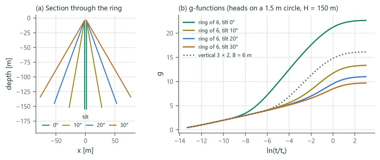
Figure 12 shows six 150 m boreholes whose heads share a 1.5 m circle. Vertical, they form a compact bundle whose g-function reaches 22.6 at = 3, more than a 3 × 2 field at 6 m spacing (16.1). Tilted outwards by 10°, 20° and 30° opposite feet lie 55, 106 and 153 m apart, and the steady g-function falls to 13.3, 11.0 and 9.7: the same length in the ground from one small drilling area interacts less than the vertical grid. Computing time (g-function at 50 times): 10 × 10 field 0.16 s vertical, 0.25 s tilted alike, 0.82 s tilted outwards (every pair its own class).
13.6 Fields of unequal boreholes
A custom layout may mix borehole lengths and radii . Each distinct gets its own (Chapter 5; grows with H through the short-circuit term). The boreholes are in parallel between the common mean fluid temperature and the field-mean wall temperature, so borehole takes and the field value is the length-weighted mean of the conductances:
is combined the same way and is length-weighted (read-outs). A field with one gets exactly the single-borehole value. The pressure drop is that of the longest loop (the shorter loops are throttled to the same flow), and the flow counts as laminar if it is laminar in any borehole. Sizing sizes the mean length and keeps the proportions,
so at fixed still depends on only through , and and the g-function cache interpolates as for an equal field; an equal field gets H in every borehole bit for bit as before. Applying a sized length to the design and the borehole-length study parameter use the same rule. Example: a 4 × 4 field with rows of 0.7, 0.9, 1.1 and 1.3 times the mean length has = 0.1172 … 0.1322 and a field value of 0.1207 m K/W; cached and exact sizing give 138.419 and 138.425 m.