The effective model of Section 3.3 gives every layer its share of the active length in three mean properties and leaves the g-function that of a homogeneous ground. This chapter describes the models that resolve the depth: the segmented layer model, in which every segment of the finite line source responds with the properties of its own layer, the borehole sections that describe the construction along the depth (diameter, grout, finite insulation), and the uniform mean fluid temperature boundary condition (UFT) that lets the section resistances act on the distribution of the heat.
11.1 Segmentation at layer interfaces and section boundaries
The segments of a borehole are those of the homogeneous engine ((4.14)), split at every layer interface and every section boundary inside :
- an interface within of a breakpoint is that breakpoint;
- otherwise the nearest interior breakpoint that is not the boundary of an end segment and has not been moved yet is moved onto the interface, if that moves it by less than half of the segment it moves into;
- otherwise the interface becomes a new breakpoint, so a thin layer gets its own thin segment; nothing is merged. The end segments keep the end-length ratio exactly, and UHTR keeps one base segment per borehole and is split only at the interfaces.
Without an interface inside the active length the segments, and therefore the g-function, are bit for bit those of the homogeneous engine.
11.2 Pair kernel
The response of receiving segment to emitting segment is the finite line source (4.4) of a homogeneous ground with the properties of the pair:
with , when both segments lie in layer . The g-function stays defined against the reference values of the effective model (, , ), so the superposition (3.6) and everything after it is unchanged; the factor converts the physical temperature into g-function units. uses and the same axial function with its mirror image, so the one-pass evaluation of Section 4.3 carries over with one lower limit per .
Why the arithmetic mean. A point source on the plane interface of two half-spaces has the exact steady temperature with . The mean also keeps symmetric in the two segments, so the reciprocity (4.9) and the symmetric job structure (and cost) of the homogeneous engine are kept. The obvious alternative is the emitter's layer (Abdelaziz et al. 2014; Erol & François 2018). Against the finite-volume reference of Section 11.5 the emitter's layer deviates by 1.25 % (two layers) and 3.64 % (three layers, strong contrast) at 50 years, the pair mean by 0.58 % and 2.23 %; the harmonic mean gives 1.35 / 3.82 %, the geometric mean 0.96 / 3.00 %.
Limits. Heat that crosses an intermediate layer between two segments sees only the two end layers, and the long-time response of a thin poor layer between good ones is overestimated (in the kernel it cannot spread vertically into its neighbours): the remaining deviation grows with time (2.2 % at 50 years for 3.0 / 1.2 / 2.8 W/(m K)).
Short times. The thresholds and of (4.18) use the smallest and the largest of all segments, and the self response of (4.19) becomes the length-weighted
The cylindrical correction (4.22) of a segment uses its own , and .
11.3 Borehole sections
A borehole design may carry sections that describe the construction along the depth, independently of the ground layers: each section has its own borehole diameter, grout conductivity and grout heat capacity, and optionally an insulation; gaps between sections use the design values, and sections outside have no effect. Insulation is always a finite resistance:
- Pipe sleeve of thickness and conductivity on all legs, the down-going or the up-going legs (coaxial: the inner pipe or both pipes). It adds to the fluid-to-pipe resistance of the pipe and enlarges its outer radius in the multipole geometry to ; a sleeve of pipe material equals a thicker pipe wall exactly:
- Casing, an insulating shell between the grout and the ground. The grout then fills (the multipole boundary lies there) and every pipe's heat crosses the shell:
is unchanged by a casing for symmetric leg layouts.
11.3.1 Two-channel conductances and the sectioned effective resistance
With summed over the legs of the down-going channel D and the up-going channel U, the conductances per metre of the two channels to the wall and between them are
( is the direct conductance of the delta circuit; it is negative when the legs lie close to the borehole wall.) With the wall at the leg temperatures of a uniform-wall-temperature borehole follow
with and . Section by section the solution is the matrix exponential , propagated upward from the bottom (the stable direction); it gives and
One symmetric piece reproduces (5.22) to . For a uniform heat flux (the classic form) the wall temperature follows from , so and is quadratic in on each piece; is evaluated exactly (Simpson's rule per piece) and one piece reproduces (5.21) to for every pipe type.
Coaxial exchangers. (5.22) assumes two channels with the same resistance to the wall. The exact coaxial solution (11.8) lies 20 % above it at 0.05 l/s and 0.3 % at 1 l/s. A coaxial design without sections keeps (5.22) (unchanged results); with sections the exact solution is used.
Results by section. The reported resistances are and as length-weighted parallel means and from (11.9) (or the fixed value); the results by section list every section and gap of the active length with , and its share of the heat (from the segment heat rates of the g-function solution at its last time). Insulated return leg: insulating the up-going leg in the top 30 % lowers where the thermal short-circuit dominates, always for the inner pipe of a coaxial exchanger (300 m, 0.5 l/s: 0.195 → 0.150 m K/W) and for a single-U only at low flow in a deep borehole (300 m, 0.1 l/s: 0.513 → 0.344 m K/W). At ordinary flows (150 m, 0.5 l/s) it raises , because the return leg also loses its own exchange with the ground.
11.4 Uniform mean fluid temperature (UFT)
Under UBWT all segments share one wall temperature, so a section resistance cannot change where the heat goes. Under the UFT condition every segment exchanges heat with one mean fluid temperature through its own local resistance (the of its section), and the coupling row of (4.16) becomes
where is the number of boreholes the segment represents. One diagonal term is added to the UBWT matrix; its size and the solver stay the same. The result is an effective-wall g-function:
It tends to 0 at short times like any wall g-function, so the short-time handling, the evaluation rules and the sizing cache apply unchanged (the g-function is marked as an effective-wall response that already contains ). The simulation uses with from (3.6) and the sectioned ; without short-circuit (large flow) this is the of the UFT solution exactly. Bounds (verified): gives the UBWT g-function, the UHTR one, and grows monotonically with in between. An insulated section receives a reduced, never zero, heat rate, and its share tends smoothly to 0 as (PU foam sleeves of 20 mm on both legs between 50 and 80 m: 0.197 of the heat per metre of the bare part).
Radius along the depth. A section with its own diameter gives its segments that radius: the self-term distance and the short-time response use the receiver's , so is no longer symmetric and every ordered segment pair gets its own entry (the Equivalent method then falls back to Similarities). This happens whenever the g-function is segmented at the sections (segmented ground or UFT); otherwise the g-function uses the length-weighted mean radius over the active length and the simulation warns.
11.5 Examples and verification
| Ground and layer model | model | [°C] | [W/(m K)] | / [°C] | Sized H [m] |
|---|---|---|---|---|---|
| Homogeneous (λ = 2.6 W/(m K)) | – | 10.73 | 2.600 | −2.41 / 16.03 | 143.7 |
| Five layers, effective model | active-length average | 11.07 | 2.621 | −1.92 / 16.34 | 140.3 |
| Five layers, effective model | mid-depth | 10.72 | 2.621 | −2.27 / 15.99 | 143.1 |
| Five layers, segmented model | active-length average | 11.07 | 2.621 | −2.00 / 16.34 | 140.9 |
| Five layers, segmented model | mid-depth | 10.72 | 2.621 | −2.35 / 15.99 | 143.7 |
| Clay over rock, effective model | active-length average | 11.62 | 2.620 | −1.38 / 16.89 | 136.1 |
| Clay over rock, effective model | mid-depth | 10.72 | 2.620 | −2.28 / 15.99 | 143.3 |
| Clay over rock, segmented model | active-length average | 11.62 | 2.620 | −1.65 / 16.91 | 138.3 |
| Clay over rock, segmented model | mid-depth | 10.72 | 2.620 | −2.56 / 16.01 | 145.8 |
Table 18 and Figure 10 show what the layering changes. With the same mean conductivity the effective model gives the homogeneous g-function; the segmented model lets the rock below 70 m take more than its thickness share of the heat, and the g-function of the clay-over-rock ground is up to 5.6 % higher at long times. The segmented field therefore needs 138.3 m instead of 136.1 m (active-length average ). The larger effect comes from the undisturbed temperature: the poorly conducting clay raises under the active-length average by 0.90 K, which shortens the heating-dominated design by 7.2 m. On the five-layer ground both effects are small.
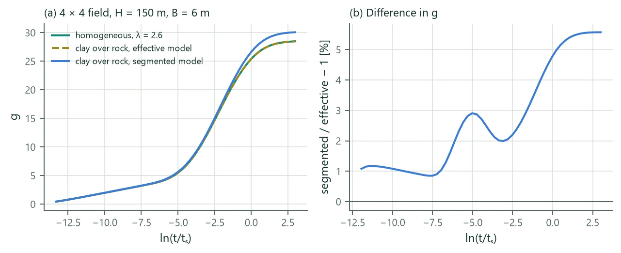
Verification. An independent axisymmetric finite-volume solution of one borehole (H = 100 m, D = 4 m, uniform flux on the wall, 26 000 cells) is the reference. BoreTherm's segmented UHTR g-function with the cylindrical correction agrees with it within 0.02 % for a homogeneous ground, 0.58 % for two layers and 2.23 % for three layers with a strong contrast (all at 50 years; 0.12 % and 0.30 % at 9 months). The sectioned resistances reproduce Hellström's closed forms to , a casing the analytic shell resistance to ; sections that repeat the design values give bit-identical results.