Both study engines run the simulation (Chapter 8) or the sizing (Chapter 9) many times on modified copies of the project; they add no physics. The program shows the results as line, heat-map, tornado, histogram, sensitivity and convergence charts and can apply the length at 95 % confidence to the design; the study setups are stored with the project.
10.1 Parameter registry
Every study input is a registered scalar with a stable identifier (ground conductivity, thickness of layer i, borehole spacing, heating-load scale, …), read and written in SI units, with a display unit and sanity bounds. A value outside the bounds makes that run fail with a message, never the study. Parameters that do more than assign a value: the borehole length sets the mean length (unequal lengths scale in proportion); the spacing regenerates a generated layout with and scales a custom layout about its centroid; the load scales multiply the energies (or all peaks). Applying a parameter's current value leaves the project unchanged bit for bit.
10.2 Parametric study
A range is an explicit list or up to . A full grid of up to three parameters runs every combination, the last parameter varying fastest:
A one-at-a-time study runs the project itself, then each parameter's values with the others at their project values, ; the spread of a result over one parameter's runs is its bar in a tornado chart. In Size mode every run is a sizing (Chapter 9), in Simulate mode a simulation at the current lengths. For the example, a conductivity sweep from 1.5 to 4.0 W/(m K) in Size mode gives 178.1 m down to 117.3 m per borehole.
10.3 Sampling
Samples are drawn by inverse transform, . With Latin-hypercube sampling (McKay et al. 1979), for each input an independent random permutation of and a uniform jitter place exactly one sample in each of equally probable strata:
Truncation to samples the truncated distribution exactly and keeps the strata equiprobable:
| Distribution | a, b, c | Inverse CDF |
|---|---|---|
| Normal | mean μ, sd σ | |
| LogNormal | median m, | |
| Uniform | min a, max b | |
| Triangular | min a, mode b, max c | for , else |
The N × k matrix of samples is drawn serially from one 64-bit Mersenne Twister seeded by the user before any run starts, with uniform variates from its top 53 bits and integers by rejection (not the implementation-defined distributions of the language's standard library). The samples, and therefore the results, are the same on every compiler and for any number of threads. Target rank correlations between inputs are imposed by the Iman–Conover method (1982): van der Waerden scores are reordered so that their Pearson correlation is
and each input column takes the ranks of its score column; the marginal distributions and the LHS strata are unchanged.
10.4 Statistics
Percentiles interpolate linearly between the sorted results (Hyndman & Fan 1996, type 7):
Mean, sample standard deviation, P5 … P95 are taken over the successful runs. In Size mode P90 and P95 of are the lengths that meet the limits with 90 % and 95 % confidence under the stated input uncertainty. Histograms use the Freedman–Diaconis bin width . The sensitivity ranking is Spearman's rank correlation, the Pearson correlation of the ranks , with ties at their average rank:
A percentile from runs is itself uncertain. The distribution-free confidence interval between the order statistics and (1-based) has the coverage
For N = 1000 and p = 0.95 the 95 % interval is … , that is P93.7 … P96.4.
10.5 Example and cost
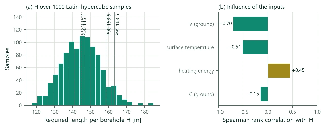
The Monte Carlo example of the office project stores a setup of 1000 Latin-hypercube samples (seed 1) in Size mode with four uncertain inputs: the ground conductivity N(2.6, 0.3) W/(m K) truncated to [1.5, 4.0], the heat capacity U(2.0, 2.6) MJ/(m³ K), the surface temperature N(9.0, 0.5) °C and the heating energy T(0.9, 1.0, 1.15) times the design value. Figure 9 shows the result: H has a median of 145.1 m (the mean inputs give 143.7 m), P90 = 158.6 m and P95 = 163.5 m per borehole, with 0 failed runs. The rank correlations with H are −0.70 for λ, −0.51 for , +0.45 for the heating energy and −0.15 for C. In Simulate mode, at the design length of 150 m, the same inputs meet the limits with a probability of 68 %.
g-function memo. Most inputs (loads, SPF, limits, fluid, pipes, grout, , ) do not change the g-function, which dominates a monthly simulation. In Simulate mode the runner therefore computes each distinct g-function once: runs that share the geometry, the g-function options and the whole ground model share an exactly computed g-function (bit-identical results); runs of one geometry that differ only in share one g-function tabulated over the union of their ranges and rescaled through (0.5–2.2 mK difference, measured). The segmented and advective models are excluded. Size mode uses the sizing's own g-function cache. The 1000-sample analysis above took 9.9 s (Size mode, all threads); in Simulate mode it takes a fraction of a second.