9.1 Objective
Sizing finds the borehole length (equal for all boreholes, positions fixed) such that the mean fluid temperature stays within . The violation
is positive where the limits are violated, and the smallest in with is sought. enters through (, , and ), (eq. (5.21)), (eq. (3.2)) and . The limit that is active at the solution is reported as the limiting condition. In a field of unequal boreholes is the mean length and the boreholes keep their proportions ((13.7)); with layered ground , and are recomputed at every trial length.
9.2 Root finding
is continuous and, for realistic cases, decreasing in . After bracketing (), the root is found with Brent's method (Brent 1973, zeroin): inverse quadratic interpolation or secant steps, safeguarded by bisection, to a tolerance of 0.1 m. The feasible end of the final bracket is returned.
9.3 g-function cache
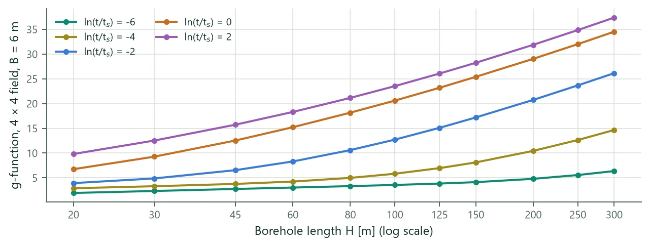
Computing the exact g-function at every iteration is the dominant cost. By default BoreTherm computes exact g-functions in parallel at five lengths spaced geometrically over ,
all on one grid of values with the spacing of (4.24). During the search is interpolated at fixed with cubic Lagrange polynomials in over the four nearest nodes, as in Peere et al. (2021). Figure 8 shows why this works: at fixed , varies smoothly with . Below a node's first time the infinite line source continues the curve:
The root of the interpolated problem is then confirmed with the exact g-function and polished by Newton or secant steps on exact simulations (usually one) until an exact point is feasible and within the tolerance; the reported length and simulation are therefore exact. If the exact and interpolated roots differ by more than 5 % or five exact steps do not converge, sizing is repeated with the exact g-function at every iteration (also selectable as an option). Measured on the example and on 10 × 10 fields (H = 60–280 m), the cached search gives extreme temperatures within 0.1 K of the exact ones (sized H within 0.4 %). For the example both variants give H = 143.7 m (12 simulations of which 2 exact, against 8 exact). The cache adds a node wherever crosses a layer interface; with groundwater flow it uses 9 nodes (g depends on H also through the Péclet number, Chapter 12); on the segmented ground 9 nodes with linear stencils inside the pieces keep the extremes within 0.1 K; with sections under UFT the exact g-function is used.
| Step | H [m] | [°C] | [°C] | g-function |
|---|---|---|---|---|
| 1 | 20.000 | −63.246 | 49.251 | interpolated |
| 2 | 300.000 | 5.388 | 15.248 | interpolated |
| 3 | 279.530 | 4.703 | 15.198 | interpolated |
| 4 | 149.765 | −2.411 | 16.024 | interpolated |
| 5 | 132.857 | −4.076 | 16.460 | interpolated |
| 6 | 143.780 | −2.984 | 16.164 | interpolated |
| 7 | 143.616 | −3.000 | 16.168 | interpolated |
| 8 | 143.628 | −2.999 | 16.168 | interpolated |
| 9 | 144.347 | −2.929 | 16.149 | interpolated |
| 10 | 142.910 | −3.069 | 16.186 | interpolated |
| 11 | 143.628 | −3.006 | 16.180 | exact |
| 12 | 143.718 | −2.998 | 16.178 | exact |
Table 16 shows the procedure on the example: the ends of the range, eight Brent steps on interpolated g-functions, and two exact simulations; the second exact point is feasible and within 0.1 m of the root.
9.4 Last-year sizing and non-monotonic cases
The classic monthly method sizes on the last simulated year only. BoreTherm checks all years by default; with the last-year option the violation (9.1) uses and of (8.6) for the last year instead:
The option acts on the exact and the cached sizing paths, the sizing trace, the sizing curve and the optimizer. BoreTherm's last year is the last operating year, which equals the classic method's calendar year when the start month is January. The difference matters when the first years are critical: in case 3 of Ahmadfard & Bernier (2019) the classic method gives 87.8 m over 10 years (and misses the first-year limit) but 112 m for a one-year run. BoreTherm gives 110.9 m by default and 88.9 m with the last-year option.
The classic-method preset combines the classic convection (5.5), the classic peak response (8.5) and (9.4). Table 68 (Appendix A) lists the measured agreement with published results of the classic method.
With a geothermal heat flux, can be non-monotonic in because rises with depth (eq. (3.2)); in the Linden worked example of the classic method's manual is violated both below the design length and above about 300 m. A -limited sizing can also be ill-conditioned ( of the order of 0.002 K/m). The trace of all evaluated lengths shows such cases.
9.5 Layout optimization
The optimizer finds the cheapest or shortest layout on a rectangular plot:
- Enumerate every layout of the selected types (line, L, U, open rectangle, rectangle, and optionally single, L2 and circle) that fits the plot in either orientation, for spacings on a grid (coarse 5 m steps when no spacing step is given), within the allowed borehole count. Mirror duplicates ( against ) are skipped.
- Screen: size each candidate in parallel with the equivalent-borehole g-function and a sizing tolerance of max(0.5 m, tolerance), within the allowed depth range.
- Refine (automatic spacing): around the ten best feasible candidates, try spacings ±1 … ±4 m in 1 m steps with the same shape.
- Rank by the objective and re-size exactly the best candidates with the project's own g-function settings, where is the number of layouts to keep; return the best .
The cost of a candidate with boreholes of length is
where is the length of the minimum spanning tree of the borehole heads (Prim's algorithm, ), an estimate of the connecting trench. The total-length objective ranks by instead. For the example plot (40 × 30 m) the optimizer screened and re-sized the candidates in 0.6 s (219 layouts screened in 0.5 s, 29 re-sized exactly; total 0.6 s). With a site plan the same search runs inside the drilling areas, with placed layout types and fill patterns as candidates and the trench to the connection point (Chapter 16).