A thermal response test (TRT) injects a heat rate into a test borehole through the circulating fluid and records the inlet and outlet temperatures. The evaluation estimates the ground conductivity and the effective borehole resistance (optionally , and a Darcy velocity) and writes them into the design project. Reference standards: VDI 4640 Part 5 (2020), ISO 17628:2015 and the ASHRAE Handbook. The program leads through the evaluation in six steps (import, setup, quality, evaluation, comparison, apply) and writes a TRT report with the contents of VDI 4640 Part 5.
17.1 Data, cleaning and quality checks
The records (time, , , flow, optional measured power and optional mean fluid temperature, for example a DTS depth mean) are never modified; cleaning only sets flags. The mean fluid temperature is unless given; the power is measured, or
with the fluid properties at the record's mean temperature; a sample's value holds over the interval that ends at it. The heating ends at the last sample above half the typical heating power. Spikes are found by a Hampel identifier (±7 samples, 4 × 1.4826 × MAD and at least 0.1 K or 5 %) on complete windows only, so genuine steps are never flagged; spikes and user-excluded intervals are left out of the fits, but their heat stays in the load history. Table 23 lists the quality checks; a failed check is reported as a failure of the test data, and every limit is editable.
| Check | Default | If violated | Source |
|---|---|---|---|
| Heating duration | ≥ 48 h | Fail | VDI 4640-5, ISO 17628; ASHRAE ≥ 36–48 h |
| Power: sd / mean (10-min means, first hour excluded) | ≤ 1.5 % | Fail | ASHRAE |
| Power: largest deviation / mean | ≤ 10 % | Fail | ASHRAE |
| Specific heat rate | 30–80 W/m | Warning | ASHRAE 50–80 W/m; VDI 4640-5 |
| Flow: sd / mean | ≤ 5 % | Warning | good practice |
| Reynolds number at the mean flow | ≥ 2300 | Warning | turbulent flow recommended |
| Days between grouting and test | ≥ 5 d | Warning | ASHRAE |
| against | ≤ 2 K | Warning | plausibility |
| Energy balance: measured power against (17.1) | ≤ 10 % | Fail | sensor consistency |
| Data gaps (spacing > 3 × median) | longest ≤ 1 h, share ≤ 5 % | Warning | good practice |
| Heating interruptions (Q < 50 % of the median) | none | Warning | M1 invalid across them |
| Spikes removed | ≤ 1 % of the samples | Warning | – |
17.2 Forward model
For a heat rate per metre that changes by at the mean fluid temperature is
with the response of one borehole at its wall: the infinite line source (4.20) (ILS, the default and reference model); the hollow infinite cylinder source (CHS, of (4.23), tabulated with a relative error below ), in which the heat enters the ground at and the borehole itself stores no heat; the finite line source (FLS) of one segment of length H at depth D, which is the line source with end effects only; and the moving line source of M3. is after a first-order lag of time constant (default 1 h), which represents the delay of fluid and grout: . The sum is a causal convolution on a uniform grid (at most 16 384 steps) evaluated with the FFT, so one model evaluation costs .
Why the line source is the reference. At the wall the hollow cylinder differs from the line source by
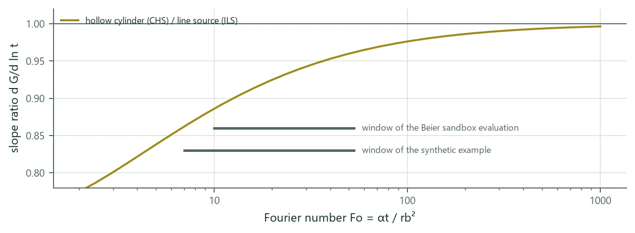
which decays only like : the slope of against is 11 % below that of the line source at Fo = 10, 8 % at 20, 4 % at 50 and 1 % at 250 (Figure 15, exact quadrature; the expansion (17.3) gives 13, 8, 4 and 1 %). Over the usual windows (Fo ≈ 5–250) a CHS fit therefore reads λ 4–9 % lower than an ILS fit of the same data, whatever the lag, the window, and the power history. A real borehole is not hollow: its core (fluid, pipes, grout) stores heat. For a perfectly conducting core of heat capacity per metre (Carslaw & Jaeger 1959, §13.7; Blackwell 1954) the slope relative to the line source is:
| 0 (hollow = CHS) | 0.5 | 1 | 1.5 | 2 | |
|---|---|---|---|---|---|
| Beier sandbox, Fo 10–53 | 0.934 | 0.961 | 0.989 | 1.018 | 1.047 |
| synthetic example, Fo 7–53 | 0.927 | 0.957 | 0.987 | 1.018 | 1.050 |
| Darmstadt logger, Fo 5–248 | 0.953 | 0.972 | 0.992 | 1.012 | 1.032 |
Usual boreholes have ≈ 0.8–1.5 (water 4.2, pipes 1.8, grout 1.5–3.9 MJ/(m³ K) against 2.0–2.6 in the ground), where the line source is within ±2 % of the core model and the hollow cylinder 5–7 % off. The line source represents the borehole's own heat capacity implicitly, the CHS neglects it; this is why the ILS is the reference model.
17.3 Methods M1, M2, M3 and M5
M1, line-source slope (Mogensen 1983). For and constant power, (17.2) with the ILS becomes , and
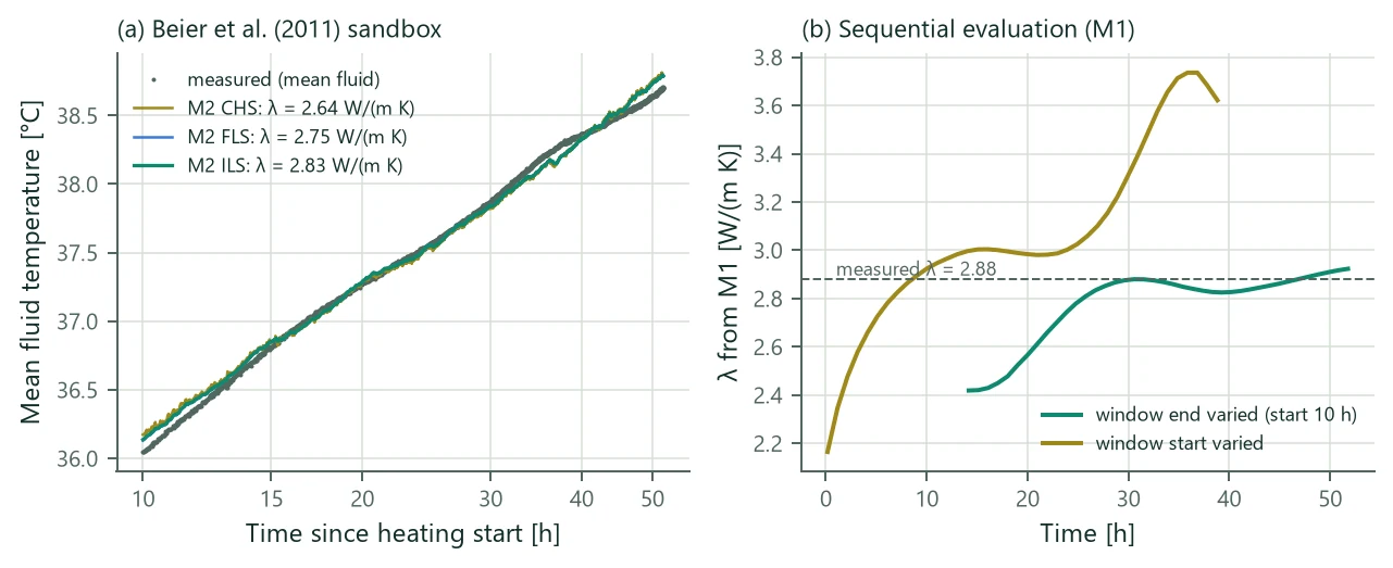
and come from least squares over the evaluation window (default from to the heating end); their covariance gives the standard errors by the delta method and 95 % intervals with the Student t quantile. The sequential evaluation repeats M1 for 40 window ends and 40 window starts (exact individual regressions by prefix sums); when rises by more than 5 % over the last half of the window ends, M3 is suggested (a drifting power has the same signature). M1 needs a constant power: a 12 % drift biases it by 5–7 %.
M2, parameter estimation with superposition. , (optionally and ) minimise over the window (and the recovery when included) with (17.2) and the chosen , by Levenberg–Marquardt with box bounds through a logistic transformation (λ 0.1–20 W/(m K), −0.2–2 m K/W, C 0.2–8 MJ/(m³ K), ± 50 K), started from M1. The covariance at the solution
gives standard errors, intervals and the correlation matrix. They assume independent residuals; real TRT residuals are strongly correlated (lag-1 autocorrelation = 0.93–0.99), so the intervals are optimistic and the Monte Carlo analysis covers the systematic input errors. The effective number of independent observations (the AR(1) variance-inflation factor) is reported with every fit:
Identifiability (every method). A fit is not identifiable, and is then shown as a sensitivity but never recommended automatically, when a parameter is at its search bound; when λ and its level parameter (, for M5 ) have (they are always strongly correlated, ρ ≈ 0.98–0.99); when any other pair has (C trades against λ through α, against ); when the 95 % interval of λ is wider than ±20 %; and, for M3, when the advection effect is below 0.05 or the interval of includes 0.
M3, moving infinite line source (Diao et al. 2004; Molina-Giraldo et al. 2011; Wagner et al. 2013). With groundwater flow the mean of the MILS temperature over the wall is
It is the ILS for and tends to . M3 estimates λ, and from three starting values of . The flow direction cannot be identified from one borehole, and a bounded test domain also looks like advection.
M5, recovery. The classic form after a heating period with mean power assumes a constant power, the logarithmic kernel and the line source:
BoreTherm superposes the whole heating history with the exact kernel of the model chosen for M2:
which is linear in and for a given ( is updated by fixed-point iteration). The recovery has no term. On cylinder-source data with 24 h of recovery the classic form read +15.6 %; the decomposition in Table 25 shows that the kernel is the cause (the recovery samples lie at Fo ≈ 7–17 since the stop, where the kernels differ most), so M5 is only as good as the kernel it uses.
| Data, power | Classic (17.8) | Log kernel + power history | Superposition, ILS kernel | Superposition, CHS kernel |
|---|---|---|---|---|
| ILS, constant | +2.6 % | +2.6 % | 0.0 % | −13.5 % |
| ILS, swing + stop | +1.6 % | +2.6 % | 0.0 % | −13.5 % |
| CHS, constant | +16.8 % | +16.8 % | +14.1 % | 0.0 % |
| CHS, swing + stop | +15.6 % | +16.8 % | +14.2 % | 0.0 % |
17.4 Undisturbed temperature and uncertainty
is the mean fluid temperature of the circulation before the heating, a manual value, or the mean of a measured temperature profile over ; without it M2 estimates and M1 gives no . The Monte Carlo analysis draws N Latin-hypercube realisations (the sampler of Chapter 10) of normal input errors (power or flow, the offsets of the two sensors, H, , C, ; defaults 2 %, 1 %, 0.05 K, 0.5 m, 2 mm, 10 %, 0.2 K) and re-runs M1 and the recommended fit on each perturbed data set, in parallel and deterministic for a seed; the result is P5/P50/P95 of λ and .
17.5 Recommended value
A fit that is not identifiable by its own diagnostics is a sensitivity: shown, marked, never chosen automatically. The rule:
- User choice: the preferred fit, if it succeeded (also when not identifiable; the reason says so).
- M2 forward model: among the identifiable M2 fits the line source is the reference; the FLS or the CHS replaces it only when it fits significantly better by the Bayesian information criterion with the effective number of observations:
with from (17.6) (the larger of the two fits) and the number of additional parameters (0 between M2 models, 1 for M3). With = 0.93–0.99 the 2000–4000 observations of a TRT count as 10–150 independent ones; a plain RMSE comparison or an F-test on would call every small improvement significant. 10 is “very strong” evidence on the scale of Kass & Raftery (1995).
- M3 replaces the chosen M2 fit when it is identifiable (including ) and (17.10) holds against it with = 1.
- Otherwise the chosen M2 fit; otherwise M1 if identifiable; otherwise M5 if identifiable.
- Otherwise nothing is recommended, and applying a result needs an explicit choice.
The reason text names the rule that applied, with ΔBIC and , and the notes list the fits set aside. M5 is the independent check, not a candidate, while M2 succeeds.
17.6 Examples
| Data | Method | λ [W/(m K)] | Δλ | [m K/W] | Δ | RMSE [K] | |
|---|---|---|---|---|---|---|---|
| Synthetic example (cylinder-source data) | M1 line-source slope | 2.715 | 4.4 % | 0.0917 | 7.9 % | 0.636 | 2 |
| M2 superposition (ILS) | 2.829 | 8.8 % | 0.0956 | 12.4 % | 0.097 | 49 | |
| M2 superposition (CHS) | 2.599 | −0.1 % | 0.0850 | 0.0 % | 0.017 | 1498 | |
| M2 superposition (FLS) | 2.820 | 8.5 % | 0.0955 | 12.3 % | 0.097 | 49 | |
| M3 moving line source (sensitivity) | 2.829 | 8.8 % | 0.0956 | 12.4 % | 0.097 | 49 | |
| M5 recovery (CHS) | 2.593 | −0.3 % | – | – | 0.014 | 421 | |
| Beier et al. (2011) sandbox | M1 line-source slope | 2.923 | 1.5 % | 0.1579 | −4.3 % | 0.036 | 29 |
| M2 superposition (ILS) | 2.831 | −1.7 % | 0.1548 | −6.2 % | 0.053 | 14 | |
| M2 superposition (CHS) | 2.639 | −8.4 % | 0.1457 | −11.7 % | 0.060 | 18 | |
| M2 superposition (FLS) | 2.746 | −4.6 % | 0.1536 | −6.9 % | 0.051 | 15 | |
| M3 moving line source (sensitivity) | 2.140 | −25.7 % | 0.1372 | −16.8 % | 0.033 | 33 |
On the synthetic example, whose data were generated with the cylinder source, the rule finds the CHS (ΔBIC 159 over the ILS with 46 effective observations) and recovers λ and within 0.1 %; M5 with the CHS kernel reads −0.3 %. On the Beier sandbox (a 18.3 m borehole in a 1.8 m box, heater power 1056 W) the line source is kept: the FLS fits slightly better but not significantly (ΔBIC 0.9), and the CHS worse. M3 has the lowest RMSE but λ and u are correlated (ρ = −0.96): the bounded box looks like advection, so M3 is a sensitivity only. The Monte Carlo analysis (200 samples) gives P5–P95 of λ = 2.68–3.00 W/(m K) for the recommended fit. Figure 16 shows the fits and the sequential evaluation. On the Darmstadt MD-BTES test (750 m coaxial borehole; Seib et al. 2025) the recommended M2 (ILS) gives 2.277 W/(m K) and 0.0547 m K/W against the paper's 2.28 / 0.05; the data set is not distributed with BoreTherm, and only these numbers are quoted.
17.7 Applying the results to the design
Applying a result writes the chosen fit into a project and lists every change. λ goes to the homogeneous ground, to every layer, or to one layer ; is the effective value over the test length, so when the effective value is to be matched, layer gets
with the length shares of (3.3), so that the project's effective conductivity over the test length equals . C is written only when it was estimated. The undisturbed temperature shifts the surface temperature so that the undisturbed temperature over the test length equals . The effective resistance is written either as a fixed value (classic style: it no longer varies with the design flow and length) or, recommended, as the grout conductivity that makes the multipole of the test borehole at the test flow and mean fluid temperature equal the TRT value; decreases monotonically with , so the root is bracketed on [0.05, 20] W/(m K) and found by the Illinois method in . The design then computes for its own flow and length. The Darcy velocity of M3 is stored on request in the ground's groundwater input, and the design simulation then uses it (Chapter 12).
Import. Delimited text files (CSV, TXT, Modelica tables) with detected delimiter and decimal comma, columns by letter, number or header, units per column, date-time formats (ISO, German, US), repeated time stamps averaged or spread, and presets for published data sets; wide DTS files (fibre positions × time stamps, several GB) are streamed one fibre position at a time (a 1.5 GB file takes about 10 s).