The usual design model treats the inside of a borehole as one thermal resistance. The fluid, the pipes and the grout store no heat, so a change of the load reaches the fluid temperature in full at once. That is accurate when the load changes slowly compared with the thermal time constant of the borehole, which is a few hours. With hourly loads, short peaks, a pump that switches on and off, or an inlet temperature that is prescribed over time (a thermal response test, a heat pump model, a thermal store), the heat stored in the borehole and the time the fluid needs to pass through it matter. The dynamic borehole model resolves the inside of the borehole for these cases. The ground outside the borehole wall stays the analytic g-function response of the field.
This chapter describes the three borehole models, the network of the dynamic model, its coupling to the ground, how hourly loads and sizing work with it, and what it changes against the steady model in a worked example.
18.1 Three borehole models
In the steady model the mean fluid temperature follows from the borehole wall temperature and the heat rate per metre (positive into the ground) through the effective borehole resistance , at every time:
contains the borehole resistance between the fluid and the wall and the thermal short-circuit between the legs through the internal resistance (Hellström 1991). Two further models add the heat capacity of the borehole interior; the model is chosen on the Design limits & simulation page.
| Model | Inside the borehole | Loads | Typical use |
|---|---|---|---|
| Steady | one resistance , no storage | monthly, hourly, time series | design of heating and cooling fields |
| Short-time capacity | the steady model plus one combined short-time response of fluid, pipes and grout | monthly, hourly, time series | hourly designs with short peaks; energy piles |
| Dynamic | fluid cells that move with the flow, grout nodes on depth levels, transit time, flow schedule | hourly or time series | verification of an hourly design, pump on/off, prescribed inlet temperature, thermal stores |
18.1.1 The short-time capacity model
The short-time model keeps everything the steady model computes and adds a correction for the heat capacity of the borehole. The pipes of a U-tube borehole are replaced by one concentric equivalent pipe that keeps the fluid and pipe-wall volumes and the film and wall resistances of the legs in parallel (Xu & Spitler 2006); its grout annulus gets the conductivity that makes the total resistance equal to , so the long-time end of the model is the steady model. A one-dimensional radial finite-volume model of fluid, pipe wall, grout and ground is run for a unit step load twice, with and without the capacities of fluid, pipes and grout. The difference is the capacity correction
with a blend weight that is 1 up to a quarter of the blend time (100 h for boreholes) and falls smoothly in to 0 at . The combined response of a unit step is
where is the g-function of the field (Eskilson 1987), the ground conductivity and the undisturbed ground temperature. In the hourly simulation the correction enters as a short convolution of the load steps with over less than 100 hours, so the steady part of the calculation is untouched. At 100 h the capacity effect is below 0.3 % of the response, and from on the model is the steady one. With all capacities set to zero the correction is exactly zero.
18.2 The cross-section network on depth levels
The dynamic model cuts the active length into levels of equal height (default = 2 m). Every level carries the thermal resistance–capacity model (TRCM) of Bauer et al. (2011): every leg of a U-tube has a fluid node and a grout node ; the fluid exchanges heat with its grout node, the grout node with the borehole wall, and the grout nodes with each other:
with the film and wall resistance of the pipe, the grout resistance of the leg and the position of the grout node. Bauer et al. derive and the grout–grout resistance from two-pipe line-source formulas. Here they are derived from the multipole resistance matrix of the cross-section, so that the steady network reproduces it exactly. With (the heat from the legs is ), , and the Laplacian of the grout–grout conductances, eliminating the grout nodes gives , hence
and . For a single U-tube this is Bauer's . The grout node sits at Bauer's position, the radius that halves the grout area of the equivalent annulus ( the borehole diameter, the outer pipe diameter, = 2, 4, 6 legs):
The network must respect the second law: and must be positive definite and every . Otherwise is reduced to (Diersch et al. 2011) until they are. A grout–grout conductance may be negative (legs close to the wall) as long as stays positive definite. Capacities per metre: the fluid of every channel and the grout of every grout node; the pipe walls carry none, as in Bauer et al. A coaxial borehole has the chain inner fluid – annulus fluid – grout node – wall, with an inner-pipe-wall node without capacity that splits in half.
Borehole sections along the depth (other diameter, grout or insulation) act per level: the network of every construction is averaged onto the levels it overlaps, weighted by the overlap length, and the heat capacity of a pipe sleeve or casing is added to the grout nodes it sits with. The film resistances depend on the flow; the level parameters are computed at relative flows of the nominal flow and cached, and with the pump off the film resistance of a laminar flow of of the nominal flow is used.
18.3 Fluid transport: plug flow without numerical diffusion
Every flow path (a U-tube: down one leg, through the U-bend and up the other) carries fluid cells of equal volume that move with the fluid: cell occupies the path volume with . Advecting a volume moves only ; when passes the outlet cell leaves the path (its heat is the outflow) and a new inlet cell enters. The inflow is mixed only into the partly filled inlet cell. The transport is therefore exact plug flow: a temperature front keeps its shape and arrives after the transit time , with no numerical diffusion beyond one cell. A cell exchanges heat with the nodes of the levels it overlaps, in proportion to the overlap.
A sub-step of length , with the control step (default 5 min), advects half the volume, exchanges heat for and advects the other half (Strang splitting). With the pump off . The run time is therefore set by the transit time and the length of the period, not by the control step.
18.4 Heat exchange between fluid and grout
A fluid cell of capacity coupled by conductances to node temperatures is advanced from to by a time-centred, exponentially fitted step:
For constant node temperatures this is exactly for every , with the conductance-weighted node mean, so the step never oscillates. With the Strang splitting the quasi-steady axial profile is that of the continuous equations (Hellström's exponential leg temperatures) independently of the sub-step. The grout nodes and the wall coupling are integrated with backward Euler. The fluid cells that touch only fixed nodes are eliminated onto those nodes, and the remaining banded system (grout nodes in depth order) is factorised once per sub-step, so the cost per sub-step grows linearly with the number of levels.
18.5 Coupling to the ground
The borehole wall temperature is uniform along the depth and equal in all boreholes, consistent with the g-function for a uniform borehole wall temperature (UBWT), which is used here with the cylindrical-source correction because the wall is resolved. On the control grid the wall temperature of step is
with the mean heat flux through the walls of the field over the step, taken from the grout nodes. It differs from the fluid load while the borehole stores or releases heat; once a load has been steady for a few days the two agree and the dynamic model gives the steady result. is the response to the earlier steps, kept by the load aggregation of Claesson & Javed (2012): the history is held in cells of growing width (in steps) with mean loads , and every step shifts a fraction of each cell's load on to the next, older cell:
where is the age (in steps) of the far end of cell . The cells cover the run plus one more level of cells, and the last cell keeps all the load it receives (no outflow), so every step conserves the energy of the load history exactly; what remains is the smearing error of the aggregation itself, a few of the response for a constant load.
With a prescribed load, the field inlet temperature and the wall temperature are the unknowns that couple all boreholes. Every node temperature is carried as an affine form , and the three parts are solved with one factorisation. In every sub-step the fluid balance of the field,
is affine in and and gives exactly, without iterating on a lagged outlet. At the end of the step the scalar equation (18.8), with affine in , gives , and every node is resolved. With a prescribed inlet temperature the load follows instead.
Boreholes in series and parallel groups of the connection network are chained: the outflow of a stage, mixed over its boreholes, is the inflow of the next. Boreholes with equal length, depth, radius and flow are simulated once and weighted by their number, so an all-parallel field of equal boreholes costs one borehole.
18.6 Flow control, pump off and fluid properties
- Inlet. Either the ground load is prescribed (hourly loads held constant within the hour, time series as row means over the step) and the inlet temperature follows, or the inlet temperature is prescribed from a time series and the load follows.
- Flow. Constant (the project flow); on/off by load (the pump stops while the load is below a threshold and runs for at least a minimum time once started); or from a time series.
- Pump off. No advection; the stagnant fluid exchanges heat with the grout and the grout with the wall; exactly. Loads requested while the pump is off are not delivered; their energy is summed and reported, with a warning above 0.5 kWh.
- Temperature-dependent fluid (option). The fluid properties, and with them the Reynolds number, the film resistances and the network of every level, are re-evaluated whenever the field mean fluid temperature moves by more than 0.5 K, so the change to laminar flow in cold periods is captured.
- Periods. The dynamic model runs over the whole period, over the first and the last year, or over custom periods. A period that starts after begins one day earlier as a warm-up, initialised from the steady state. Outside the dynamic periods the steady model runs on the same grid and pushes its loads into the same aggregation, so the ground history is continuous.
18.7 Energy balance and outputs
Over the dynamic periods the program sums the energy delivered by the fluid, the energy through the walls and the change of the heat stored in fluid and grout, and reports the largest relative step error of the balance:
with the enthalpies and the stored heat taken relative to 0 °C. The Dynamic model page shows the inlet, outlet, mean fluid and wall temperatures, the wall flux, the load and the flow at the output interval, depth profiles of the down-going and up-going legs and of the grout at chosen times, and the flow direction. The hourly arrays (hour means) and a monthly view (base = the last hour of each 730-hour month, peaks = its extremes) are filled as by the other models, so the Results summary, the Mean fluid temperature page, the Annual page and the limit check work unchanged.
18.8 Hourly loads and sizing with the dynamic model
The dynamic model needs hourly or time-series loads. Hourly loads may be generated from the monthly table: the generator keeps the energy and the peak power of every month and spreads the rest by the outdoor temperature and a use pattern (for an office: office hours on working days). The limits are checked on the hour means of all years (or of the last year).
Size borehole length works with every borehole model: with the dynamic model it runs the dynamic model at every trial length, on the same cached g-functions as the steady sizing. That is accurate but slow. The faster route is to size with the steady model and then run Verify with dynamic model on the Required borehole length page: it copies the project, sets the boreholes to the sized length, switches to the dynamic model with the project's dynamic settings and runs it together with the steady model at the same length. The project itself is not changed. The result shows the hour-mean range against the limits, the range at the output interval (more extreme when the control step is shorter than an hour) and the steady range.
18.9 Example: an office field with hourly loads
A small office with a ground-source heat pump: 200 MWh/year space heating (peak 100 kW), 8 MWh/year domestic hot water and 45 MWh/year cooling on 16 boreholes of 150 m in a 4 × 4 grid, ground conductivity 2.6 W/(m K), over 25 years; the limits are −3 / 20 °C. The monthly loads are turned into hourly loads with the office pattern. Table 28 lists the runs.
| Loads and run | Borehole model | [°C] | Length H [m] |
|---|---|---|---|
| Monthly loads, 150 m | steady, monthly | −2.41 | – |
| Monthly loads, Size borehole length | steady, monthly | −3.00 | 143.7 |
| Hourly loads, 150 m | steady, hourly | −3.06 | – |
| Hourly loads, Size borehole length | steady, hourly | −3.00 | 150.7 |
| Verify at 150.7 m | short-time capacity | −2.92 | – |
| Verify at 150.7 m | dynamic | −2.89 | limits met |
| Hourly loads, Size borehole length | dynamic | −3.00 | 149.5 |
Hourly loads make the field 7.0 m per borehole longer than the monthly sizing (112 m in total): the office draws its heating peak for a whole working day, day after day, while the monthly method assumes a 6-hour peak on top of the monthly mean. The dynamic model at the hourly length keeps 0.11 K above the limit, so the steady length is confirmed with a small reserve. Sizing with the dynamic model gives 149.5 m, 1.2 m shorter (0.8 %), from 10 dynamic runs of 25 years each.
Figure 17 shows why the difference is small. In the first hour of the coldest 12-hour load block of the last year the steady model drops by the full , to −1.68 °C; the dynamic model reaches only −0.87 °C, because the fluid and the grout give off stored heat first. The coldest hour, however, is the last one of the block, when that storage is spent: there the models differ by only 0.11 K (−3.00 against −2.89 °C). The dynamic model matters most for short peaks; for long load blocks the steady length is close. The depth profiles show the fluid warming on its way down and up, with the grout between fluid and wall; the difference between the legs is the thermal short-circuit that accounts for in the steady model.
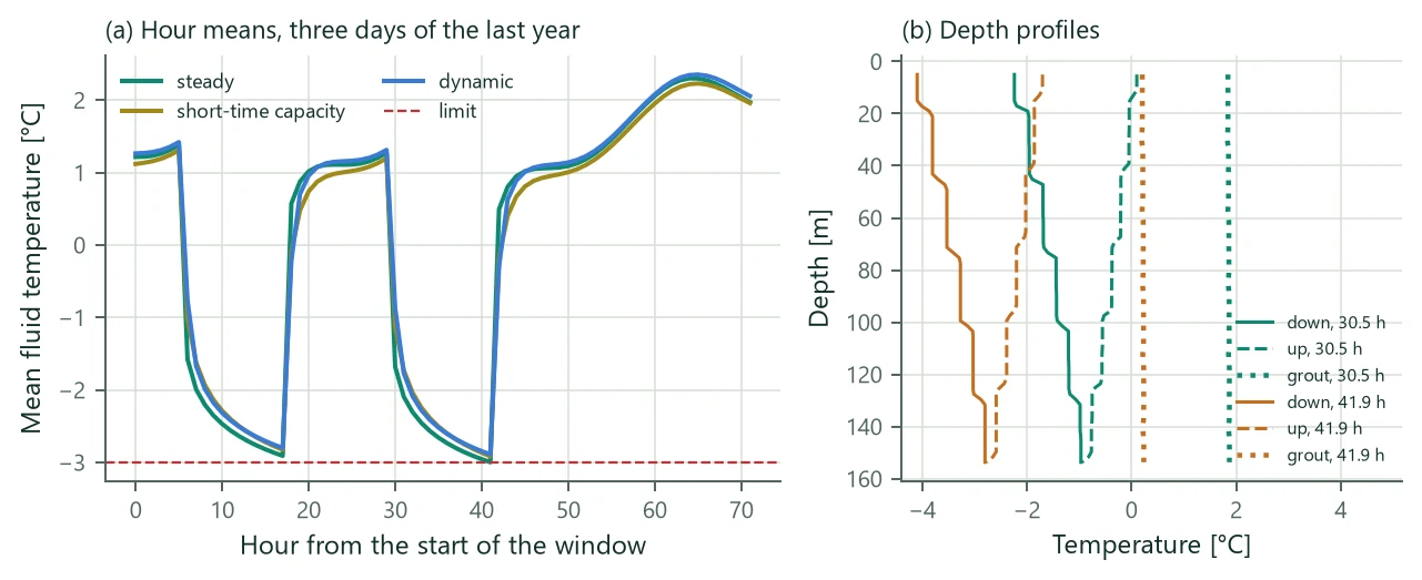
Discretisation of the run: 75 levels of 2.01 m, control step 300 s, sub-step 32.5 s. Over 25 years the fluid took 2463 MWh from the ground and 2463 MWh passed through the walls; the largest step error of the energy balance (18.11) is . The lowest inlet temperature is −4.18 °C with the steady model and −4.09 °C with the dynamic model.
18.10 Verification
- Quasi-steady limit. Without grout capacity and with loads held constant for a month, the fluid temperature of the dynamic model follows the steady relation (18.1) within 2.0 mK at the default 10 sub-steps per transit (0.63 mK with 20), and the steady model within 3 mK.
- Transit delay. A step of the inlet temperature from 10 to 20 °C in a 50 m borehole with insulated pipes arrives at the outlet as a step from 10.000 to 19.998 °C within one cell and two control steps of the transit time: no numerical diffusion.
- Laboratory data. The sandbox thermal response test of Beier, Smith & Spitler (2011), 18.3 m single U-tube over 52 h, run with the measured inlet temperature: outlet temperature RMSE 0.155 K, maximum 0.286 K after the first hour.
- Short-time against dynamic model. Pulses of 5 kW for 3 h every 12 h over 10 days: the two capacity models agree within 0.134 K, while the steady model is 0.886 K away. After 460 h of constant load the dynamic model is 4.0 mK from the steady model.
- Energy balance. The step error (18.11) stays below for single boreholes, boreholes in series and 3 × 3 and 10 × 10 fields over a year, with the pump switching on and off.
- Periods. In the steady year of a first-and-last-year run the result equals the hourly steady model within 0.9 mK: the ground history carries the wall fluxes of the dynamic year.
The network itself goes back to Bauer et al. (2011) and Pasquier & Marcotte (2012); the multipole-derived parameters reproduce Hellström's steady leg temperatures and the effective resistance along the depth.
18.11 Limits
- Hourly or time-series loads are needed. Generated hourly loads are synthetic: they keep the monthly energies and peaks, not the real weather.
- The limits are checked on hour means; with steps shorter than an hour the series at the output interval can be more extreme.
- In the basic ground coupling the wall temperature is uniform along the depth and equal in all boreholes. Coupling per ring or per borehole exists for thermal stores (next chapter); vertical stratification is not resolved.
- A 25-year run takes a minute or more, and sizing runs it at every trial length. The first-and-last-year option is much faster.
- The dynamic model is not available for energy piles (its network does not resolve the concrete core) or for spiral coils.