A borehole thermal energy store (BTES) is a compact borehole field that is charged with heat in summer and discharged in winter. Hot fluid enters at the centre while charging; for discharging the flow is reversed, so that cooler fluid enters at the edge, picks up heat ring by ring and leaves through the hot centre. The store keeps a radial temperature gradient, hot in the middle and cooler towards the edge, where the heat losses happen. The design question is not whether a fluid temperature stays within limits, but how much of the stored heat comes back, and at which temperature.
The program simulates a store with the dynamic borehole model of the previous chapter, extended by the operation (inlet temperature, flow and flow direction over time), a ground coupling that gives each ring or each borehole its own wall temperature, flow reversal through the same pipes, and a yearly storage summary.
| Heating and cooling field | Thermal energy store | |
|---|---|---|
| Loads | monthly or hourly ground loads | a time series of inlet temperature, flow and direction; the load is a result |
| Borehole model | steady, optionally short-time capacity | dynamic (transit time, depth levels, grout capacity); the steady pipe model in between |
| Ground | one wall temperature for the field | one wall temperature per ring or per borehole |
| Flow | one direction, pump always on | reversed for discharging; pump off in rest periods |
| Main results | , , required length | charged and discharged heat, recovery per year, outlet temperatures, ring temperatures |
19.1 The operation series
The operation is a time series with a constant step. Every row holds the inlet temperature (or the ground load), the flow and the flow direction (+1 as the connections are drawn, which is the charging direction; −1 reversed; 0 keep the previous direction). A series that covers one year repeats every year. The flow is stored as given, so that it stays right when the fluid or the connections change later, and converted at run time. A mass flow becomes a volume flow with the density of the fluid at the inlet temperature of the step,
and a flow per borehole (the mean flow through one of the boreholes) becomes the pump flow of the network through
with the borehole flows of the network at its nominal total flow and the flow-weighted mean number of boreholes in series that a fluid particle passes: for an all-parallel field, for pairs in series, for a ring-wise string of stages. The total of the borehole flows is then for every network.
When no measured series exists, the Generate BTES operation dialog builds one year (365 days from the start month, repeated) at a step between 5 min and 1 h. Every calendar month is Charge, Rest or Discharge. Inside the daily operating hours of a charging month a row gets direction +1, the charging flow and the charging inlet temperature (or a positive load); a discharging month gets direction −1, the discharging flow and inlet temperature (or a negative load); otherwise the pump is off. With a prescribed load the energies of a year are known in advance, and with the operating rows. The dialog can switch the borehole model to Dynamic with the inlet, flow and direction taken from the series.
19.2 Ground coupling per ring or per borehole
The basic dynamic model gives every borehole the same wall temperature. A store lives from the opposite, a hot centre and a cool edge. The ground coupling therefore partitions the boreholes into groups with their own wall temperature, uniform along the depth:
- Uniform (default): the whole field, .
- Per ring: the convex-hull layers of the borehole heads, innermost first. On hexagonal and concentric layouts these are the symmetry classes; on rectangular grids a hull layer mixes corners and edges, which per ring averages.
- Per borehole: every borehole; for networks without symmetry. Above 300 boreholes the program asks for a confirmation, because the cost grows with the square of the number of groups.
The group response is the length-weighted mean wall-temperature rise of group caused by a unit heat rate per metre on every borehole of group , in units of :
with the segment-pair integrals of the finite line source (with groundwater the moving finite line source, also for inclined boreholes and layered ground) for a uniform heat rate, and the cylindrical-source correction on the self terms. The responses satisfy, to rounding,
(the field-mean response is the uniform-heat-rate g-function; reciprocity holds without groundwater, and with groundwater after reversing the flow direction). Curves that are equal by symmetry are stored once: a hexagonal field of 19 boreholes coupled per borehole has 9 distinct curves of 361 pairs.
Every source group keeps its own load history in aggregation cells , and every distinct curve its difference table . The history term of group is
and at the end of a step the wall temperatures follow from one dense linear system,
where is the heat through the walls of group over the step (affine in the wall temperatures and the inlet temperature, as in the uniform model) and the length of the group. A node of a borehole is affine in its own group's wall temperature and in everything that reaches it with the fluid: the inlet temperature and the walls of the groups upstream in its string. With a prescribed load the inlet temperature is one more unknown, closed by the energy of the step. The energy balance of every step holds as in the uniform model.
Steady model per group. Outside the dynamic periods (and for a fast hourly run of the whole period) every borehole is a steady two-channel pipe model at its group's wall temperature, and . Chained along the strings, the heat rate of every group is linear, , and with the ground
Both models push their group loads into the same aggregation, so the ground history is continuous across the periods. At slow loads the steady model follows the dynamic one within 0.01 K.
19.3 Flow reversal
The network as drawn is the normal, charging direction (the store layouts put the inlet at the centre). Reversed runs every string backwards: the normal outlet stage becomes the inlet stage, and every borehole is entered through its other channel (for a U-tube the up-going legs become the down-going ones; for a coaxial borehole annulus-in becomes centre-in). A switch moves no fluid. The path is measured from the other end, and cell at offset is the same piece of pipe as cell at offset with
with the number of cells of the path. The cells are only re-indexed: each keeps its temperature, place and volume, the stored heat is unchanged, and the next advection moves them the other way, so the fluid that entered last leaves first. The direction of a step with flow is
- Fixed: always normal;
- From the time series: the sign of the direction column over the step;
- Automatic: with a prescribed inlet temperature, normal when is at least above the fluid of the normal inlet stage, reversed when it is at least below the fluid of the normal outlet stage, otherwise unchanged; with a prescribed load, normal for injection and reversed for extraction. Defaults = 1 K and at least 1 h between two switches;
- Time series, then automatic: the column where it is non-zero, the rule elsewhere.
Charging fluid hotter than the centre thus enters there, and discharging fluid colder than the edge enters at the edge. With the pump off the direction is kept.
19.4 Storage results
The Storage page shows one row per operating year (8760 h from the start of the simulation, so a year begins in the start month). With the heat the fluid gives to the ground in a control step of length (> 0 into the ground):
summed over the steps with flow of the year. The cumulative recovery is from year 1. Further results: the hours charging, discharging (by the sign of , not by the schedule) and with the pump off; the number of direction switches; the minimum and maximum inlet and outlet temperatures with flow; and, with a coupling per ring or per borehole, for every ring the length-weighted mean wall temperature at the end of the year's last charging and last discharging step and the wall heat split by its sign. The ring wall heat differs from and by the heat stored in fluid and grout. The values are taken per control step, so an output interval that mixes charging and discharging does not net them.
All heat the fluid exchanges with the ground counts: there is no useful-heat threshold or return-temperature cut-off, so the outlet temperatures have to be judged together with the recovery. In a storage operation the program warns when the inlet or outlet temperature exceeds , which here also stands for the limit of the pipe material (about 90 °C for PE-RT or PE-Xa), and when the fluid reaches its upper property limit (water 100 °C).
19.5 Example: a hexagonal store of 37 boreholes
37 boreholes of 50 m, 3 m apart in a hexagon of 4 rings, connected as six strings that run ring by ring from the centre outwards. Charging May to September at 70 °C, discharging November to March at 30 °C, pump off otherwise, 0.25 kg/s per borehole of water; ground conductivity 2.0 W/(m K), undisturbed temperature 10.0 °C; 3 years from April, control step 1 h. The series prescribes the inlet temperature, the mass flow per borehole and the flow direction; the coupling is per borehole. The steady model per borehole runs the whole period hourly, and the dynamic model runs from day 940 to 954 (with one day of warm-up before).
| Year | Charged [MWh] | Discharged [MWh] | Recovery [%] | Cumulative [%] | Hours charging / discharging / off | Switches | [°C] |
|---|---|---|---|---|---|---|---|
| 1 | 580 | 92 | 15.9 | 15.9 | 3889 / 3407 / 1464 | 1 | 29.9 – 62.3 |
| 2 | 426 | 138 | 32.5 | 22.9 | 3672 / 3624 / 1464 | 2 | 30.6 – 63.9 |
| 3 | 401 | 152 | 37.9 | 27.2 | 3672 / 3624 / 1464 | 2 | 30.8 – 64.2 |
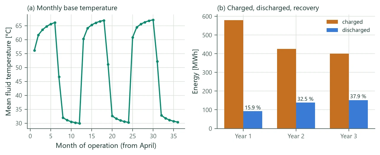
Table 30 and Figure 18 show the typical start-up of a store. A new store must first warm its own ground and the ground around it, and that heat does not come back in the first winter: year 1 recovers 15.9 %, year 3 37.9 %. Over the 3 years 1407 MWh were charged and 382 MWh discharged. Year 1 counts 217 h more charging than the schedule: at the end of the first winter the store has cooled to about the discharge temperature (outlet 29.9 °C), so the 30 °C inlet is warmer than the ground and . The mean fluid temperature ranges from 10.0 to 67.1 °C; the minimum is the undisturbed ground before the first charge.
| Ring | Boreholes | end of charging [°C] | end of discharging [°C] | Wall heat in [MWh] | Wall heat out [MWh] | Out / in [%] |
|---|---|---|---|---|---|---|
| centre | 1 | 67.0 | 32.0 | 10 | 6 | 59 |
| 1 | 6 | 66.5 | 31.7 | 59 | 33 | 56 |
| 2 | 12 | 64.6 | 31.2 | 122 | 56 | 46 |
| 3 | 18 | 59.7 | 30.5 | 210 | 57 | 27 |
Table 31 shows why the coupling per ring matters. The centre loses heat only to its warm neighbours, the outer ring to the cold ground outside, and it returns the least. With the uniform coupling this radial difference is averaged away.
Recovery is not a property of the store alone. It depends on the operation: the discharge temperature sets how far the store can be cooled, so a lower discharge temperature gives a higher recovery. Every kilowatt-hour that cannot be taken out above the discharge inlet temperature stays in the ground.
19.6 Verification
The coupling per ring and per borehole and the flow reversal were compared with an independent finite-element code that resolves every borehole in three dimensions: seven single-U boreholes of 50 m (a centre and a ring of six at 5.2 m), charged for 120 days at 70 °C and discharged for 150 days at 15 °C, all in parallel or as a ring-wise string with the discharge reversed. The numbers below are from the verification report.
- Outlet temperatures: within 0.09 K (parallel) and 0.12 K (ring-wise string) after the first ten days of each period with the coupling per ring or per borehole. The uniform coupling misses the centre outlet by 0.69 K, because one wall temperature cannot give the centre its warmer wall.
- Charged heat: within −1.1 to −1.6 % (parallel) and −1.4 to −1.9 % (string), meeting the 3 % target.
- Discharged heat: −4.3 % over the year and −6.5 % for 30-day cycles (parallel, per ring), outside the 3 % target; the uniform coupling gives −7.3 %, and −38 % on the centre borehole. For the cycles the deficit lies almost entirely in the first day after each switch, where the near field of the reference model lags (−0.01 % without the first 1.5 days of every period); for the year, about half of it comes from the borehole resistance: with matched to the reference it falls to −2.2 %. The discharged heat is about 15 % of the charged heat, so 3 % of it corresponds to a mean outlet offset of about 0.03 K.
- Internal checks: per ring and per borehole agree with the uniform model on symmetric two-borehole fields to K; the energy balance holds across direction switches to about relative; per ring and per borehole on hexagonal fields of 19 and 37 boreholes agree within 0.008 K on the outlet.
19.7 Limits
- The wall temperature of a group is uniform along the depth: vertical stratification in the store and a thermal insulation on top of it are not resolved. Insulated pipe sections (sleeves, casings) act on the levels of the borehole model.
- Outside the dynamic periods the steady pipe model has no transit time and no grout capacity. For cycles of days, run the dynamic model over the whole period.
- Judge a store on its later years; year 1 always includes the heating-up of the surroundings.
- Size borehole length sizes the length to the fluid temperature limits only; there is no sizing for a recovery target. Compare variants (length, spacing, temperatures) with Calculate runs.
- No useful-heat threshold: heat discharged at a temperature the plant cannot use still counts.