A ground-source heat pump pays more at the start and less for energy every year. Whether that pays off depends on the period, the interest rate, the tariffs, the maintenance and the residual value of the long-lived borefield, not on the seasonal performance factor alone. The heating-system comparison compares the project's borefield heat pump with an air/water heat pump, gas and oil condensing boilers, a pellet boiler, district heating and an air/water heat pump with a gas peak boiler (hybrid). Every enabled variant must deliver the same useful space heating, hot water and cooling, and each one is reduced to one number: its annual full cost, the annuity of all its discounted cash flows over the period, in the manner of VDI 2067. A ground-source system can lose the comparison.
The example is an office building (about 3000 m²) with monthly loads of 200 MWh/a space heating, 8 MWh/a hot water and 45 MWh/a cooling on a 4 × 4 field of 16 boreholes of 150 m, compared over 20 years at 2 % interest with gross real prices (EUR 2026), the residual value credited, no grant, and the synthetic climate of central Germany (mean 10 °C, amplitude 9 K, design outdoor temperature −12 °C). Tariffs and plant costs of the data set are illustrative values flagged as assumptions.
29.1 Service and energy of each variant
The service comes from the building loads of the project, monthly or hourly; multiyear load tables are averaged to one year, which the economics repeat. Projects with ground loads entered directly cannot be compared, because the useful heat and cold cannot be reconstructed from them. Monthly loads are spread over the hours with the load generator where a variant needs hourly demand.
- Ground-source heat pump. The borefield simulation of the project gives, month by month (hour by hour with hourly loads), the brine leaving the field, , as the source and the heating-curve flow (or the DHW temperature) as the sink. The COP comes from the heat pump model; load above the capacity, or brine below the minimum source temperature, goes to an electric backup at COP 1; the source pump runs its hours. Passive cooling is used while the brine of the peak injection case stays at or below the passive limit (16 °C by default), active cooling with the EER above it. If the cooling of the variant differs from that of the design, the field is simulated again for the requested cooling.
- Air/water heat pump and hybrid. Hour by hour from the synthetic outdoor temperature: the COP at the outdoor and flow temperature, the capacity of the machine, hot water first, and a backup heater for the rest. Below the bivalence point (−3 °C by default) the hybrid's gas boiler covers what its heat pump cannot; the hybrid's power-ratio rule is checked against the part-load capacity, not certified.
- Boilers and district heating. Fuel = useful heat / seasonal efficiency , plus auxiliary electricity. Gas is billed on the gross calorific value , oil and wood on the net value ; statutory gas factors given per kWh are divided by the ratio = 1.108 (an assumption of the data set) before they multiply the modelled kWh .
- Cooling. Reversible machines or chillers supply the same useful cold; a variant that cannot cool gets an air-cooled chiller (SEER 3.5) so that the service stays equal.
The synthetic climate is seeded: a seasonal cosine around the annual mean of the climate preset, a daily cycle of ±4 K (warmest at 15 h) and an autocorrelated day-to-day weather with a standard deviation of 3 K. It drives the air/water COP and the heating curve of every heat pump; it is not a test reference year. The energy boundary of a heat pump includes compressor, backup heater and source circulation, so its SPF is the simulated system value; the tabulated JAZ after VDI 4650 Blatt 1:2024 is reported beside it for the heat pump variants (for the borefield with the lowest field outlet temperature as the minimum brine inlet temperature and the simulated source-pump power).
29.2 Investment and operation
The borefield is priced with the cost estimate of the project (simple or detailed, at the current length) and has a service life of 50 years. The plant of every variant is priced at its design power with the cost curves of the KWW technology catalogue for heat planning, (net, for the ground-source heat pump without the borehole source, which the borefield estimate prices), plus the catalogue's additional costs (heating surfaces, buffer, chimney or fuel storage, the district-heating connection) as a separate component. Service lives, repair and servicing fractions and operating hours follow VDI 2067 Blatt 1; the borefield gets 2 % repair and 1 % servicing and inspection per year of its investment. The annual operation of a component is
with the investment C, the two VDI 2067 fractions, the operating hours h and the labour rate (zero for owner-operated residential projects). The fractions apply to the equipment only. Investment entered for a variant is net and is converted to the selected gross or net convention. All defaults are meant to be replaced by local quotations.
29.3 Discounted cash flows, net present value and annuity
With the interest rate , and the period , the initial investment and a grant are paid at , energy and operation at the end of every year , and replacements at for a component of life , each discounted at its exact time. The residual value of the last installation, made at , is its unused linear life, credited at :
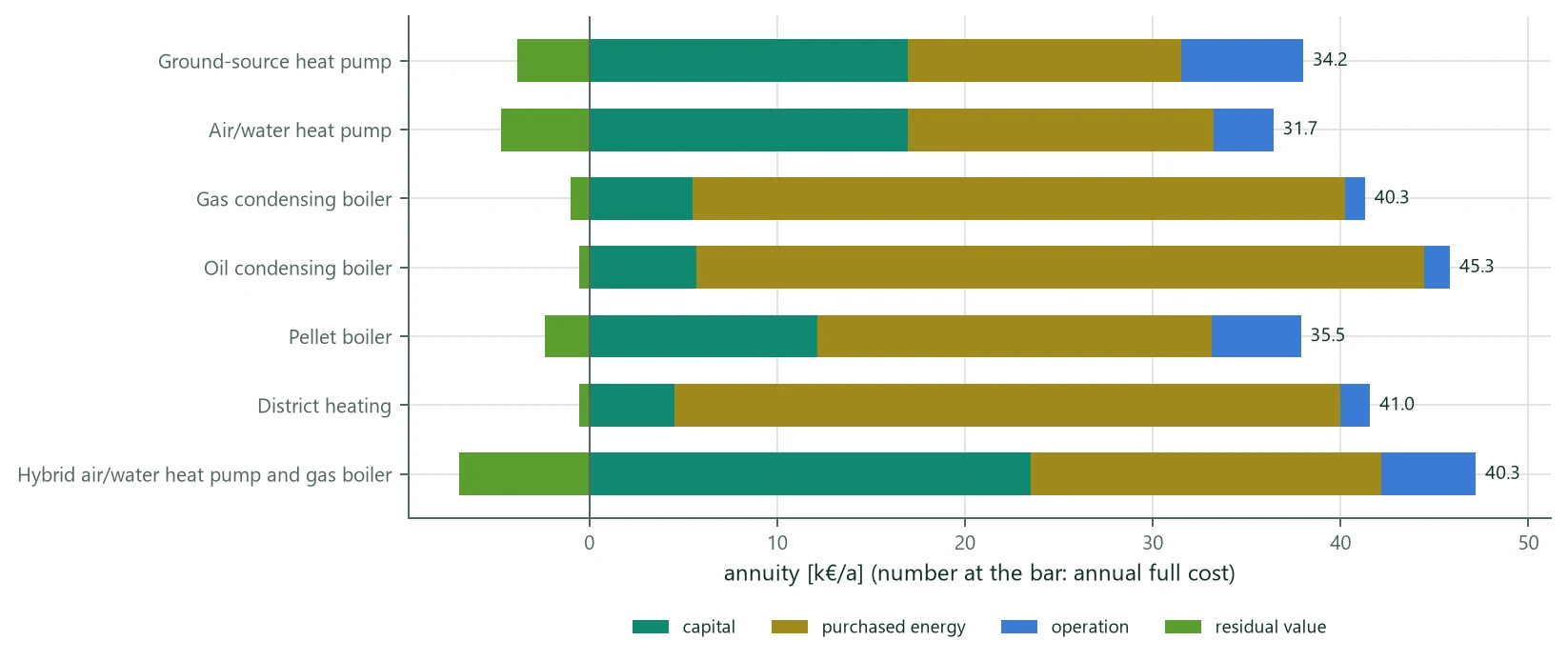
Costs are positive, grants and the residual value negative. is the annual full cost; at , . Each cost group (capital, purchased energy, operation, other, grant, residual value) is annualised from its own present value, which gives the split of Figure 25. For an energy price that escalates at a constant rate the present-value factor of the energy is
The yearly cash flows agree with these closed forms, including replacements and residual value, to a relative error below , and reproduce the published example of VDI 2067 ( = 6 %, = 2 %, = 5: = 0.237, = 4.374). With energy costs only, the ground-source system breaks even with a boiler at
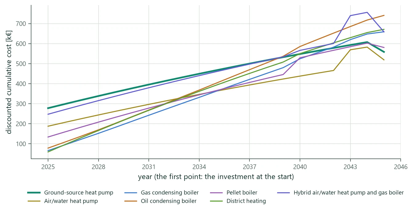
which shows why tariffs matter as much as efficiency. The break-even year is the first year after which the discounted cumulative cost of the ground-source system stays below that of the other variant to the end of the period; later replacements can move or remove it, so it is not a simple payback time.
29.4 Prices, carbon and grants
User price anchors are interpolated linearly and held at the nearest end outside their range; without a path, . Standing charges are applied once per carrier. Prices are real unless nominal prices are selected with consistent paths. For new gas and oil heating the fossil fuel is blended with renewable fuel at the steps of the German building energy law (10 / 15 / 30 / 60 % from 2029 / 2030 / 2035 / 2040), approximated as a fuel share at equal efficiency, and the carbon charge is added separately (retail tariffs must therefore exclude it):
with the combustion emission factor EF in kg/kWh and the carbon price in €/t (plus VAT in a gross comparison). Low, central and high carbon-price paths are scenarios, not legislated prices; they change only the variants that burn gas or oil. Grants are off by default. They can be a confirmed amount, a user rate and cap, or the dated automatic rules of the German federal funding programmes; the automatic estimate does not check technical, applicant or building eligibility and is assumed to be paid at the start.
29.5 Levelised cost of heat and ecology
holds the cooling energy and the components allocated to cooling (a chiller, or a cooling fraction of a shared component). Shared costs stay with heat unless allocated, which matters when passive cooling shares the borefield. Two ecological boundaries are reported as annual values at the date of the data set, not as lifetime forecasts: the statutory CO2-equivalent and non-renewable primary energy (compliance metrics of the German building energy law), and an estimate of direct fossil CO2 (grid electricity 0.344 kg/kWh, without upstream emissions, refrigerants and other greenhouse gases; biogenic CO2 counts zero). Qualitative scores with weights (noise, space, permits, drilling risk, price exposure) are a separate judgement; a knock-out removes a variant from the lowest-cost marker, and scores never change the costs.
29.6 Example
| Result | How it is derived | Example |
|---|---|---|
| Useful heat and cold | building loads | heat 208,000 kWh/a (DHW 8,000), cold 45,000 kWh/a |
| Electricity | COP at field outlet and heating-curve flow, capacity share, backup, source pump; passive cooling: the pump only | heating 44,605 kWh/a, cooling 7,297 kWh/a (source pump 13,363 kWh/a in total) |
| SPF, SEER | (27.9) | SPF 4.66, SEER 6.17 |
| JAZ after VDI 4650 | lowest monthly field outlet as minimum brine temperature | 4.53 ( 0.98 °C, 1.134) |
| Investment | plant + additional costs + borefield net total, × (1 + VAT) | (60,834 + 41,332 + 131,200) × 1.19 = 277,705 € |
| Energy cost | kWh × tariff | 51,902 kWh × 0.28 €/kWh = 14,533 €/a |
| Operation | (29.1) | 6,494 €/a |
| Residual value | (29.2) | borefield 156,128 × (50 − 20) / 50 = 93,677 € → −3,855 €/a |
| Annual full cost | (29.3) | a = 0.0612: 34,154 €/a |
| LCOH heat / heat + cold / cold | (29.7) | 15.4 / 13.5 / 4.5 ct/kWh |
| CO2 and primary energy | kWh × factor of the carrier | 29.1 t/a statutory, 17.9 t/a direct estimate, 93 MWh/a |
| Variant | Investment [€] | Annual full cost [€/a] | LCOH heat [ct/kWh] | SPF or | CO2 stat. [t/a] | Ground source cheaper from |
|---|---|---|---|---|---|---|
| Ground-source heat pump | 277,705 | 34,154 | 15.4 | 4.66 | 29.1 | – |
| Air/water heat pump | 187,690 | 31,734 | 13.7 | 4.45 | 32.5 | never |
| Gas condensing boiler | 65,941 | 40,299 | 16.6 | 0.96 | 54.2 | 2042 |
| Oil condensing boiler | 78,383 | 45,292 | 19.0 | 0.93 | 76.6 | 2039 |
| Pellet boiler | 133,785 | 35,502 | 14.3 | 0.90 | 12.0 | 2045 |
| District heating | 59,300 | 41,036 | 16.9 | 0.98 | 45.5 | 2040 |
| Hybrid air/water heat pump and gas boiler | 247,395 | 40,269 | 16.6 | – | 36.9 | 2039 |
In this example the air/water heat pump has the lowest annual full cost; the ground-source system costs 2,421 €/a more. By cost group, ground source minus air/water heat pump [€/a]: capital +17, energy −1,719, operation +3,290, residual value +833. The largest difference is the operation: the data set gives the borefield VDI 2067 repair and servicing of 3 % of its investment per year (4,684 €/a here). The ground-source system has the lower energy cost and CO2 and becomes cheaper than gas, oil, pellets, district heating and the hybrid within the period. The default tariffs and plant costs are illustrative: replace them, and review the operation fractions of the borefield, before drawing a conclusion.
29.7 Coupled heat-pump economics
With fixed seasonal performance factors the borefield temperatures come from the SPF of the loads, while the comparison computes the electricity of the ground-source variant with its own heat pump model from the simulated source temperatures; the two assumptions differ, and a warning says so. In the temperature-dependent mode the ground loads are recomputed from the COP at the simulated field outlet until the energy-weighted SPF changes by less than 0.01 (at most five passes), so the borefield temperatures and the heat-pump electricity are consistent, and the ground-source variant uses the project's heat pump and the borefield sized for it.
| Ground-source variant | Fixed seasonal efficiency | Temperature-dependent |
|---|---|---|
| Heat pump in the calculation | fixed SPF for the ground loads; default datasheet model of the variant | machine B of the heat pump chapter (2 × 60 kW, minimum brine −8 °C, EER 5.6) |
| Borehole length, borefield net total | 150 m, 131,200 € | 160.0 m, 138,415 € |
| Coupling passes | none (one pass) | 3, converged |
| SPF (simulated) / JAZ (VDI 4650) | 4.66 / 4.53 | 4.71 / 5.13 |
| Electricity [kWh/a] | 51,902 | 51,984 |
| Annual full cost [€/a] | 34,154 | 34,748 |
The plant investment of the variant stays the cost curve of the data set; the quotation of the chosen machine belongs in the variant table. Beyond one comparison the coupling serves three tools: a length sweep of the levelised cost and the SPF against the borehole length, which shows the depth dependence and the temperature-limit boundary; the life-cycle cost objective of the layout optimizer, which ranks thermally sized candidates by their annualised cost with coupled performance (it ranks candidates and does not search a continuous economic optimum over all depths); and Monte Carlo runs on a saved comparison, which carry the uncertainty of building and ground into the SPF and the cost distribution of every variant and give the probability that the ground-source system is the cheapest. That probability is conditional on the input distributions; it does not remove the uncertainty of the model or of its default assumptions.
29.8 Sensitivity
The comparison tabulates a one-at-a-time sensitivity, each case as the annual full cost of the ground-source system minus that of the cheapest other system:
- interest 1 % and 5 %; period 15 and 30 years;
- electricity and fuel prices ±20 %; the low and the high carbon-price paths;
- drilling price ±30 %; plant investment ±20 %;
- residual value off and on.
Switching the residual value off shows how much the result rests on the long life of the borefield. Scenario bands are not statistical confidence intervals; if the same explicit carbon path is given to every scenario, the bands coincide.
29.9 Limits
- The climate is synthetic, not a test reference year; it drives the air/water COP and every heating curve.
- Default tariffs, plant costs, chiller and district-heating data are illustrative; the data set flags each value with status and date and warns when values expire or are older than six months.
- With monthly loads the brine minimum of the JAZ is a monthly mean.
- The automatic grant estimate does not check eligibility; ecological values are annual values at the data date.
- The comparison covers one building. Landlord cost splits, tax credits, refrigerant leakage, groundwater, direct-evaporation and separate hot-water heat pumps and solar support are not modelled. It is an indicative comparison, not a binding offer.