4.1 Definition
Eskilson (1987) defined the g-function as the dimensionless borehole-wall temperature response of a field to a unit step heat rate applied at :
For the example, = 1.182e-06 m²/s and = 2.115e+09 s = 67.1 years. is the mean over all boreholes, and the heat rate per metre of the whole field. At short times is the response of a single borehole; the thermal interaction between boreholes makes grow with the number of boreholes and their proximity until a steady state is reached at about . BoreTherm tabulates at nodes and interpolates linearly in :
Below the first node is taken linear in from , and beyond the last node it is held at the last value (steady state). The characteristic time uses the mean borehole length.
4.2 Finite line source with mirror image
Each borehole is represented by a line source of finite length. Following Cimmino & Bernier (2014) and Cimmino (2018), the boreholes are divided into segments; the mean temperature change on receiving segment (length , top depth ) caused by a unit heat rate per metre on emitting segment (, ) at horizontal distance is, in units of ,
with for the self-response. The axial function contains the real source and its mirror image above the ground surface, which keeps the surface at :
The first four terms are the real source, the last four its mirror image. The integral in (4.4) is symmetric in and , which gives the reciprocity relation
so only one of each pair has to be evaluated. For the integral has the closed form used by the equivalent-borehole clustering (Section 4.5):
4.3 Numerical integration
4.3.1 Adaptive Gauss–Kronrod quadrature in ln s
With the substitution () the integrand of (4.4) becomes , which is smooth over the many decades of spanned by the time grid. The integral is split at the lower limits of the requested times and accumulated from the steady-state end, so that every interval is integrated once:
and . Beyond the factor is negligible. Each interval is integrated with a globally adaptive 7-point Gauss / 15-point Kronrod rule (Piessens et al. 1983): the sub-interval with the largest error estimate is bisected until every component satisfies , with times the length of the shorter segment. All distances that share one segment-pair geometry (the same ) are integrated on one mesh, because the expensive factor does not depend on the distance.
4.3.2 Cancellation-free evaluation of the erfint sum
For large every term grows linearly while their sum stays bounded; summing them directly loses all significant digits. BoreTherm uses for and sums the linear and constant parts analytically ():
The remaining terms decay instead of growing. The direct form (4.5) is used where (erfint is even, so may be used throughout).
4.3.3 Closed-form approximation (Cimmino 2021)
As an option the integral is evaluated in closed form. With erf approximated by a sum of exponentials, (, ; coefficients of Tanash & Riihonen 2020, = 10 terms by default), each term of (4.4) integrates analytically. With , and :
is evaluated by its power series for and by a continued fraction (modified Lentz) above. For the 10 × 10 field of Section 4.5 the closed form agrees with the quadrature to 0.006 % (Table 6).
4.4 Boundary conditions
4.4.1 Segmentation
For the uniform-temperature condition each borehole is divided into segments (default 8), refined geometrically toward both ends so that the end segments have the length (end-length ratio = 0.02; Eskilson 1987, as in an open-source g-function library). For even the length ratios from the top are
with the expansion factor found by bisection; odd adds a middle segment . The uniform-heat-rate condition is exact with one segment per borehole, because the FLS integral is additive over the segments of both emitter and receiver.
4.4.2 Uniform heat transfer rate (UHTR)
Every segment emits the same heat rate per metre. The segment temperatures follow without a linear solve, and is their length-weighted mean:
4.4.3 Uniform borehole-wall temperature (UBWT)
Eskilson's g-functions, and hence those of the classic monthly method, assume that all boreholes share one wall temperature (equal fluid temperature) with a prescribed total heat rate. The segment heat rates are then unknowns. At each time step of the grid the segment heat rates and the common wall temperature solve the system (Cimmino & Bernier 2014; Cimmino 2018)
where is the number of segments of the field, the matrix of response factors at the current step length (interpolated linearly in between grid times, with ), the segment lengths and the wall temperatures caused by the heat rates of all earlier steps, evaluated with :
The increments come from a load-history reconstruction (the scheme of an open-source g-function library): the history , , is re-averaged onto a reversed grid whose step durations are those of the actual grid taken in reverse order. On that grid every past step ends a grid time before , so (4.17) needs only at the grid times, already computed. The system (4.16) is solved with a dense LU factorisation with partial pivoting at every step. Because the solution superposes the segment heat rates over the grid actually requested, depends slightly on the grid: for a 3 × 2 field the value at 20 years changes by 0.02 % between 320 and 600 grid points, and by 0.3 % on an 11-point grid.
4.4.4 Short-time handling
Two short-time limits apply. Below (2.8 minutes for the example) the line source is not valid, and is taken linear in from to , as in an open-source g-function library. Second, the UBWT time stepping (4.16)–(4.17) is unstable when it starts at Fourier numbers below about 0.2: the segment self-response is then so small that the segment heat rates oscillate, and oscillates and can even turn negative (down to −25 for H = 20 m on fine grids). The same behaviour is found with that open-source library on such grids. BoreTherm therefore starts the UBWT solver no earlier than
(35 minutes for the example), 2.5 times the observed stability limit. Between and the boreholes do not yet interact and the heat rate along them is still uniform, so follows the length-weighted self-response of the boreholes, scaled to the solver value:
with the CHS − ILS difference (4.22) added to when the cylindrical correction is on (Section 4.6). This keeps positive and increasing on any time grid. In verification computations on grids starting at 60 s, a single borehole and a 3 × 3 field agree with the open-source library within above and within of its valid solution between and , and a 20 m borehole stays positive and increasing with every method and option on 1-second grids. UHTR has no time stepping and is solved down to .
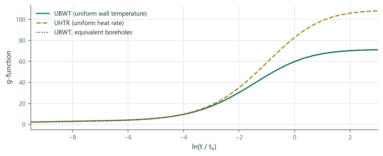
Figure 1 shows the difference between the two conditions for a 10 × 10 field: with a uniform heat rate the central boreholes become much warmer than the outer ones, and the steady-state is 106.0 instead of 70.2 at = 2. UBWT is the default and the choice consistent with the classic monthly method. A third condition, a uniform mean fluid temperature with a local resistance per segment (UFT), lies between the two and is described in Section 11.4.
4.5 Detailed, Similarities and Equivalent methods
The cost of a g-function is dominated by the number of distinct response factors. BoreTherm evaluates only the distinct entries of :
- Detailed: one entry per segment pair (halved by (4.9)).
- Similarities (default; Cimmino 2018): pairs with the same segment geometry and the same borehole-to-borehole distance share one entry. Sorted distances are grouped starting from the shortest ungrouped distance : all distances form a group represented by their mean (distance tolerance disTol = 0.01).
- Equivalent (Prieto & Cimmino 2021): boreholes are clustered by their steady-state UHTR wall temperature (eq. (4.10), summed over all emitters) with one-dimensional complete-linkage clustering, cut at the middle of the longest dendrogram branch. One equivalent borehole represents each cluster, and one entry holds the sum of all pair responses between two clusters. The size of the linear system (4.16) drops from to a few times .
| Variant (10 × 10, B = 6 m, H = 150 m) | Time [s] | at = −6 | −2 | 0 | 2 | Max. dev. [%] |
|---|---|---|---|---|---|---|
| UBWT, Similarities (default) | 0.172 | 4.197 | 30.584 | 59.972 | 70.231 | 0.000 |
| UBWT, Detailed | 0.294 | 4.197 | 30.584 | 59.970 | 70.229 | 0.003 |
| UBWT, Equivalent | 0.005 | 4.197 | 30.694 | 60.158 | 70.419 | 0.367 |
| UBWT, Similarities, closed-form FLS | 0.230 | 4.197 | 30.584 | 59.972 | 70.235 | 0.006 |
| UHTR, Similarities | 0.001 | 4.200 | 35.307 | 83.094 | 106.029 | 52.141 |
| UBWT, 12 segments | 0.364 | 4.197 | 30.567 | 59.869 | 70.069 | 0.236 |
| UBWT, Similarities + CHS | 0.177 | 4.199 | 30.584 | 59.972 | 70.231 | 62.693 |
For a 20 × 20 field (400 boreholes, 3200 segments) the default method takes 3.5 s and the equivalent-borehole method 0.011 s, with a largest deviation of 2.0 %. Refining the segmentation from 8 to 12 segments changes by at most 0.24 % for the 10 × 10 field. The equivalent method is therefore used for fast screening (the optimizer, Section 9.5) and for very large fields, and the detailed or similarities method for final results.
4.6 Short-time behaviour and the cylindrical-source correction
At short times a single borehole behaves like an infinite line source (ILS):
( = 0.5772 is Euler's constant), which Eskilson wrote in terms of as
valid for . The classic monthly method uses (4.21) for its peak pulses (Section 8.2). The line source places the heat on the borehole axis; at times of the order of (hours) the real borehole behaves like a cylindrical surface source (CHS). The optional cylindrical-source correction adds the difference CHS − ILS to the self-response of every segment (Carslaw & Jaeger 1959, §13.7):
The integral is evaluated by adaptive quadrature in ; vanishes at long times. Figure 2 compares the options for a single borehole of the example.
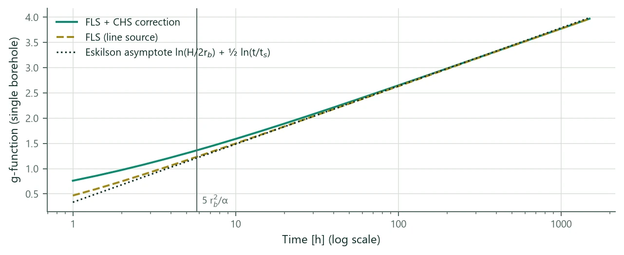
At a 6-hour peak ( = −11.49) the field g-function of the 4 × 4 example is 1.253 (identical to the single borehole: there is no interaction yet), the asymptote (4.21) gives 1.231 and the ILS 1.254. The corresponding difference in a peak fluid temperature is a few hundredths of a kelvin (Section 8.2). The CHS correction raises by 0.14 at about 6 h and is off by default, as in the classic monthly method.
4.7 Layouts
Layout generators build the field from a prototype borehole (H, D, ) and the parameters , , (along x) and (along y). The borehole order follows that of an open-source g-function library so that reference data can be compared borehole by borehole; shared corners appear once.
| Type | Definition | Boreholes |
|---|---|---|
| Single | one borehole | 1 |
| Line | boreholes along x | |
| LShape | along x and along y, sharing the corner | |
| L2Shape | L plus the same L shifted inward by one spacing (the classic L2 layout) | about |
| UShape | along x, two legs of along y including the corners | |
| OpenRectangle | perimeter of an rectangle | |
| Rectangle | filled rectangle | |
| Circle | boreholes on a circle of radius | |
| InclinedRing | heads on a circle of radius , tilted outwards (Chapter 13) | |
| Custom | CSV file with x, y [, H, D, , tilt, azimuth], drawn in the field view, or a fill of a site plan (Chapter 16) | any |
| Layout | N | at = −6 | −4 | −2 | 0 | 2 | Time [s] |
|---|---|---|---|---|---|---|---|
| Single borehole | 1 | 3.96 | 4.92 | 5.79 | 6.43 | 6.67 | 0.002 |
| Line, 10 | 10 | 4.05 | 6.26 | 10.62 | 15.42 | 17.28 | 0.005 |
| L, 6 + 5 | 11 | 4.05 | 6.36 | 11.25 | 16.66 | 18.69 | 0.006 |
| U, 6 × 4 | 12 | 4.06 | 6.44 | 11.81 | 17.75 | 19.93 | 0.006 |
| Rectangle 4 × 4 | 16 | 4.13 | 8.12 | 17.20 | 25.40 | 28.24 | 0.009 |
| Rectangle 10 × 10 | 100 | 4.17 | 9.57 | 30.36 | 59.87 | 70.23 | 0.179 |
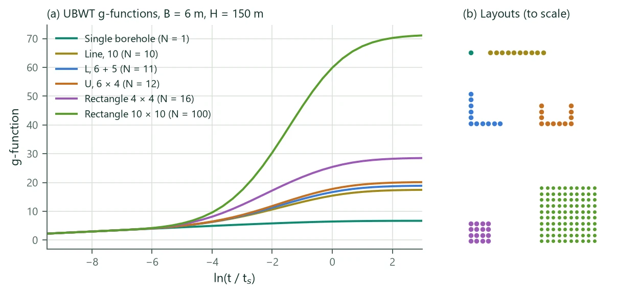
Figure 3 and Table 8 show the expected ordering: at short times every field follows the single-borehole curve; the more compact the field, the earlier and stronger the interaction. A line of 10 boreholes interacts less than an L or U with a similar count, and the 10 × 10 field reaches .
4.8 g-function times used by the simulation
The simulation computes at times spaced evenly in from half an e-fold below the shortest time needed (, the shortest peak duration or 1 h) to half an e-fold above the simulation period :
that is about four points per e-fold. Monthly and hourly responses are then interpolated with (4.3).