The borehole resistance links the mean fluid temperature to the borehole-wall temperature. BoreTherm computes it from the pipe geometry, the grout, the ground and the flow with the multipole method (Claesson & Hellström 2011) and Hellström's (1991) short-circuit formulas. This chapter treats one uniform borehole; sections with their own diameter, grout and insulation are in Section 11.3, fields of unequal boreholes in Section 13.6 and boreholes connected in strings in Chapter 14.
5.1 Pipe resistance
The resistance from the fluid to the outer wall of one pipe is the sum of convection, conduction through the wall and an optional contact resistance:
The worked example of the classic method's published manual prints the three terms separately (0.1757, 0.0771 and 0.02 m K/W), which confirms the form. Flow and convection are evaluated for one pipe: in a double- or triple-U the borehole flow is split equally over the parallel U-tubes, as in the classic monthly conventions.
5.2 Flow and convection
Default (Gnielinski). For fully turbulent flow, Re ≥ 4000 (Gnielinski 1975):
For laminar flow, Re ≤ 2300, Nu = 3.66 (fully developed, uniform wall temperature). In the transition range the Nusselt number is interpolated linearly in Re (Gnielinski 2013, eqs. 16–17):
where the friction factor inside is the one at the actual Re, as in an open-source g-function library.
Classic option. The convection model of the classic monthly method was identified numerically: the worked example of its published manual (Re = 1184, Nu = 3.999) and all ten rows of the manual's against flow (Re = 1059–10589) fit, to 0.1 %, the Colburn form without a transition blend (Hellström 1991, eq. 7.43):
With the option set, (5.5) replaces (5.3)–(5.4) for every U-tube pipe and for the inner pipe of a coaxial exchanger; the annulus keeps its own correlation (the classic one for the annulus could not be confirmed), and the friction factor, the pressure drop and the laminar flag are unchanged. The two models differ most in the transition range, where the classic form jumps to the turbulent value at Re = 2300; with the default correlation BoreTherm's differs from the classic values by 0.5–3 % in the published cases. With the classic option BoreTherm reproduces the Linden worked example of the manual (double-U, Re = 1184): = 0.2727, = 0.2088, = 0.6629 and = 0.2100 m K/W against the published 0.2728 / 0.2088 / 0.6625 / 0.2100, i.e. within 0.06 %.
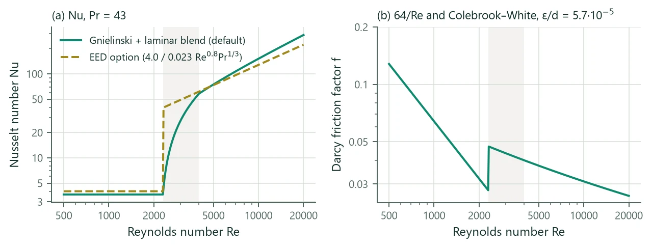
Figure 4a compares the two models. At the example's Re = 4958 they nearly coincide (Nu = 74.0 and 72.9); in the transition range the classic form gives up to about ten times the laminar value while the blend rises gradually.
5.2.1 Coaxial annulus
The annulus between the inner pipe (outer radius ) and the outer pipe (inner radius ) uses the hydraulic diameter and, for laminar flow (Hellström 1991; Çengel & Ghajar 2015),
for the inner and outer walls; Gnielinski on for turbulent flow, with the same linear blend.
5.3 Friction factor
The Darcy friction factor is for Re < 2300 and the Colebrook–White equation above, solved by fixed-point iteration on from the Swamee–Jain estimate (about ten iterations to machine precision):
For the laminar annulus the exact Hagen–Poiseuille solution is used:
5.4 Multipole method
The multipole method (Bennet, Claesson & Hellström 1987; Claesson & Hellström 2011) solves steady conduction in the borehole cross-section: circular pipes (centres as complex numbers, outer radii , fluid-to-wall resistances ) in a grout disc of radius and conductivity , surrounded by ground of conductivity . The result is the resistance matrix :
where is the heat flow per metre leaving pipe and the mean temperature of the borehole wall. With and , the zero-order (line-source) resistances are (Hellström 1991; paper eq. 33)
Multipoles of order at every pipe correct for the non-circular temperature field around the pipes. They satisfy the wall condition (paper eq. 38)
where is linear in the heat flows (the term ) and in the multipoles and their conjugates (paper eq. 34); the source term is
and the fluid temperatures follow as (paper eq. 32)
The paper and the usual open-source implementations solve (5.12) by fixed-point iteration. Because the condition is real-linear in , BoreTherm splits and solves the real system directly with one LU factorisation, shared by the unit load cases that give the columns of . The result is exact for the chosen (no convergence tolerance). = 0 reproduces the line-source formulas; the default is = 3, and up to 10 is accepted (the classic method allows 1–10).
5.5 Local and internal resistances
With all pipes at the same fluid temperature, the local borehole resistance is
The internal resistance between the down-going and up-going legs follows from the antisymmetric case: down-legs at , up-legs at , (Hellström 1991, eqs. 8.16–8.18). With the sign vector ( down, up), the pipe heat flows are and
For a symmetric single-U, (5.15) and (5.16) reduce to the classical forms
is the resistance of the Hellström model with one down and one up channel; for multiple U-tubes it is used with the heat-capacity flow of the whole borehole in the formulas of Section 5.7.
5.5.1 Leg conventions
The legs of U-tubes lie on a circle of radius , where (the shank spacing) is the centre-to-centre distance between opposite legs, as in the classic monthly method. Leg is at angle . Legs flow down and leg , diametrically opposite leg , is its return leg, so the down-legs of a double-U are adjacent (90° apart) and those of a triple-U are at 0°, 60° and 120° (Figure 5). This is the arrangement of the classic method (whose shank spacing is the distance between the two legs of one U-tube) and of the common open-source tools. With it and the classic convection option, BoreTherm reproduces the published double-U = 0.6625 m K/W (0.6629) and the manual's -against-flow table to 0.09 %.
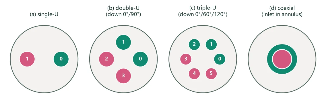
The convention matters for only; treats all legs alike. For the example double-U at 0.5 l/s BoreTherm gives = 0.2867 m K/W; an independent evaluation with the multipole routine of an open-source g-function library (J = 3, same ) gives 0.2861 with the down-legs adjacent and 0.2223 with them diagonal (0°/180°). The same routine reproduces BoreTherm's single-U and to four decimals. The network of that library for a multiple U-tube with the inlets listed first coincides with the uniform-temperature formula (5.22) for this layout.
5.6 Coaxial borehole heat exchanger
For a coaxial exchanger (an outer and an inner pipe, concentric with the borehole) the multipole correction vanishes and the resistances are analytic. With the fluid entering the annulus (default) or the inner pipe, and radii , (inner pipe) and , (outer pipe):
is here the fluid-to-fluid resistance between the inner channel and the annulus. The Reynolds number and convection reported are those of the channel the fluid enters first. The coaxial model has not been compared with published results of the classic monthly method.
5.7 Effective borehole resistance
Heat exchange between the down- and up-going legs (thermal short-circuit) raises the resistance between the mean of the inlet and outlet temperatures and the borehole wall. Hellström (1991) defines the effective resistance by
and gives two closed forms. Uniform heat flux along the borehole (Hellström 1991, eq. 8.101; the form of the classic monthly method, which reproduces the worked examples of its manual and all ten rows of the manual's table):
Uniform borehole-wall temperature (Hellström 1991, eqs. 8.87–8.88; reported to agree better with thermal response tests by Spitler et al. 2016):
with for . is the heat-capacity flow of the whole borehole (both U-tubes of a double-U). The formula is an option (default uniform heat flux). Because (5.21) depends on , is recomputed at every trial length during sizing. With a fixed effective resistance > 0 (the classic “constant values”, for example a thermal-response-test result) it is instead constant at every length, as in the classic monthly method and in all tools compared by Ahmadfard & Bernier (2019); , , , Re, Nu and the pressure drop are still computed and reported, and the input must be finite and non-negative:
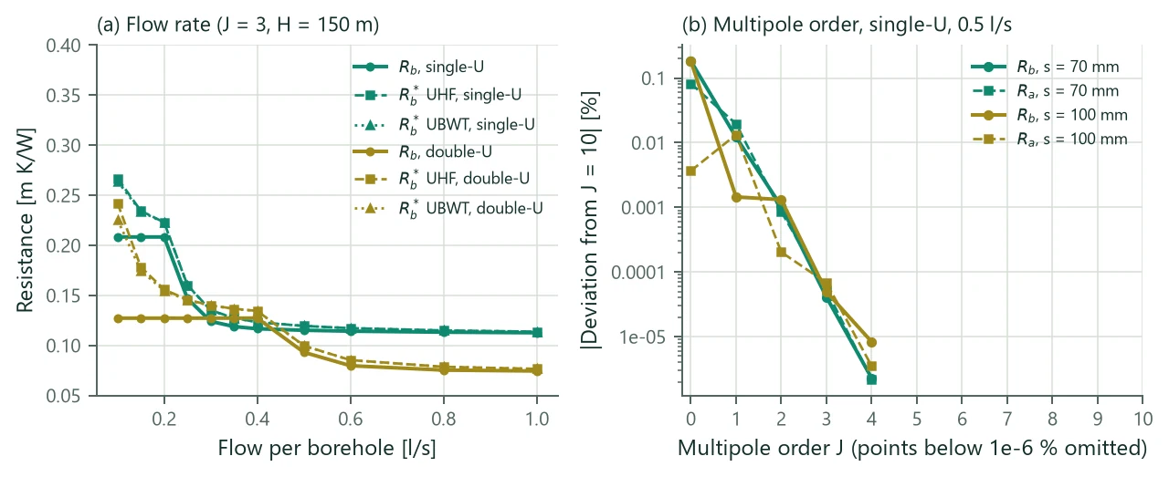
Figure 6a shows the parameter study. At 0.5 l/s (Re = 4958) the single-U has = 0.1151, = 0.4397 and = 0.1194 m K/W. Below Re = 2300 (about 0.23 l/s) the constant laminar Nusselt number freezes at 0.2083 m K/W, while keeps rising as the flow falls (0.2669 with (5.21) and 0.2639 with (5.22) at 0.1 l/s). The double-U halves the flow per pipe, so its laminar range extends to 0.46 l/s. Figure 6b shows that the multipole expansion converges very fast: = 0 is within 0.2 % and = 3 within % of = 10 for these geometries.
| Flow [l/s] | Re | UHF | UBWT | classic conv. | classic conv. | Δp [kPa] | (2U) | (2U) | ||
|---|---|---|---|---|---|---|---|---|---|---|
| 0.10 | 992 | 0.2083 | 0.8091 | 0.2669 | 0.2639 | 0.2000 | 0.2612 | 13.0 | 0.1272 | 0.2420 |
| 0.20 | 1983 | 0.2083 | 0.8091 | 0.2229 | 0.2227 | 0.2000 | 0.2153 | 26.1 | 0.1272 | 0.1559 |
| 0.25 | 2479 | 0.1468 | 0.5649 | 0.1602 | 0.1600 | 0.1189 | 0.1356 | 58.3 | 0.1272 | 0.1456 |
| 0.30 | 2975 | 0.1240 | 0.4746 | 0.1351 | 0.1349 | 0.1177 | 0.1294 | 79.4 | 0.1272 | 0.1400 |
| 0.40 | 3966 | 0.1166 | 0.4455 | 0.1232 | 0.1231 | 0.1161 | 0.1228 | 129.5 | 0.1272 | 0.1344 |
| 0.50 | 4958 | 0.1151 | 0.4397 | 0.1194 | 0.1194 | 0.1152 | 0.1195 | 189.6 | 0.0931 | 0.0997 |
| 0.60 | 5950 | 0.1142 | 0.4362 | 0.1172 | 0.1172 | 0.1145 | 0.1175 | 259.2 | 0.0797 | 0.0853 |
| 0.80 | 7933 | 0.1132 | 0.4322 | 0.1149 | 0.1149 | 0.1136 | 0.1153 | 425.8 | 0.0753 | 0.0786 |
| 1.00 | 9916 | 0.1126 | 0.4298 | 0.1137 | 0.1137 | 0.1130 | 0.1141 | 626.9 | 0.0744 | 0.0765 |
| J | single-U | single-U | double-U | double-U |
|---|---|---|---|---|
| 0 | 0.1153 | 0.4400 | 0.0907 | 0.2818 |
| 1 | 0.1151 | 0.4396 | 0.0931 | 0.2855 |
| 2 | 0.1151 | 0.4397 | 0.0931 | 0.2867 |
| 3 | 0.1151 | 0.4397 | 0.0931 | 0.2867 |
| 4 | 0.1151 | 0.4397 | 0.0931 | 0.2867 |
| 10 | 0.1151 | 0.4397 | 0.0931 | 0.2867 |
Table 9 and Table 10 list the values behind Figure 6. For the example geometry every order gives the same four printed decimals. The classic convection option changes little in fully turbulent flow (0.1152 against 0.1151 m K/W at 0.5 l/s) and in laminar flow (Nu = 4.0 instead of 3.66), but strongly in the transition range: at 0.25 l/s (Re = 2479) it gives 0.1189 instead of 0.1468 m K/W, because the classic form jumps to the turbulent correlation at Re = 2300 while the Gnielinski blend rises gradually.
5.8 Pressure drop and pump power
The friction pressure drop follows Darcy–Weisbach over the flow path of one borehole: the length of one U-tube (the U-tubes are in parallel), or in the annulus plus in the inner pipe of a coaxial exchanger:
The header pipework is not included (minor losses of the string connections: Chapter 14). With boreholes in series (the series factor of the classic method), the flow per borehole and the pump power are
For the example (16 boreholes, 0.5 l/s each, = 0.5): = 189.6 kPa and P = 3033 W. Because in turbulent flow, the pump power grows quickly with the flow while improves only slightly.