Horizontal groundwater flow carries heat away from (or towards) the boreholes. BoreTherm models it with the moving finite line source (MFLS; Molina-Giraldo et al. 2011) inside the segment-to-segment engine of Chapter 4 and Chapter 11, so layouts of any shape, unequal lengths, UBWT and the layered models work with a flow as without.
12.1 Inputs and the Péclet number
The input is the Darcy velocity (specific discharge) of a uniform aquifer or of each layer, and the flow direction (from +x counter-clockwise). Heat moves with the effective heat-transport velocity
with = 4.18 MJ/(m³ K) the volumetric heat capacity of the water and that of the saturated ground. As soon as one layer has its own velocity, the layer values replace the uniform one. The program shows Pe with the guideline of Molina-Giraldo et al. (2011): below 1.2 the flow is negligible, from 1.2 to 10 the MFLS is needed, above 10 advection dominates and the axial (finite-length) effects are negligible. For the office example (H = 150 m, λ = 2.6 W/(m K), C = 2.2 MJ/(m³ K)) 1 m/yr gives Pe = 7.6.
12.2 Kernel
The continuous moving point source (Carslaw & Jaeger 1959, §10.4) has the kernel . With the substitution of (4.4) the flow adds the factor and a direction weight. For two vertical segments at horizontal distance , the receiver lying downstream of the emitter (, ):
with the same ((4.5); the mirror image moves with the same flow, so the surface stays isothermal). gives the FLS bit for bit. Numerics. The engine integrates and puts the rest, , into the component weights: and are huge and tiny at high Péclet numbers, their product is not. A distance contributes where ; below
every kernel is negligible, has reached its steady state and those time intervals are skipped. The kernel of one distance is a bump at about wide in ; the integration intervals are split at the bumps so that the adaptive Gauss–Kronrod rule cannot step over one on a coarse time grid.
Self term. The receiver is the borehole wall () and the wall points lie at ; the mean of over the circumference gives the self weight (at borehole scale for m/s). Closed-form limits used in the verification: the steady state of the infinite line (MILS) and its transient form (Diao et al. 2004),
12.3 Pair classes, methods and layered aquifers
- The integral of a segment pair is still symmetric; only the direction weight distinguishes receiver a / emitter b from the reverse, so reciprocity becomes . Detailed keeps one class per ordered borehole pair and .
- Similarities groups distances as in Cimmino (2018), but at most disTol· apart, so that the direction factor of a class is off by at most about disTol; within a distance group the pairs are sub-grouped by and split by the sign of x (downstream, upstream, across the flow).
- The jobs (segment pairs) stay unordered, so the cost is that of the conductive model (10 × 10 UBWT: 0.158 s with flow against 0.153 s without). Equivalent falls back to Similarities (its clustering uses the conductive steady state, which the plume does not follow); the approximate FLS has no advective form and is refused with groundwater. UHTR keeps one segment per borehole.
Layered aquifers. Each layer has its own . A segment pair in one layer uses that layer's value; a pair in two layers uses, consistently with (11.2), the mean Darcy flux:
With the effective model the thickness-weighted mean Darcy velocity over the active length is used with . An aquifer confined to one layer lies strictly between the conductive and the fully advective g-function, as verification computations confirm; no independent three-dimensional reference with layered flow was available, so the pair velocity is an approximation of the same kind as (11.2).
12.4 Simulation, sizing and studies
- , , and are those without flow (the grout is not flowed through); only changes. The short-time handling is unchanged: at borehole scale the flow is negligible for hours to days.
- Sizing: at fixed , now depends on H through Pe (the advective time is fixed). It stays smooth in , and the g-function cache uses 9 nodes with cubic stencils: on the office example the interpolated extremes of are within 0.09 K ( m/s) and 0.03 K ( m/s) of the exact simulation over 35–270 m, against 0.12 / 0.23 K with 5 nodes.
- Study memo (Chapter 10): rows with groundwater share g-functions only exactly (same ground model including , and the direction); no rescaling through .
- The classic monthly method has no groundwater model; the program and the report say so.
12.5 Example: the office field in an aquifer
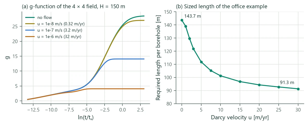
Figure 11 and Table 19 show the groundwater variant of the office example with a uniform flow along the rows. The field's g-function saturates earlier and lower as the flow grows: the plume carries the heat away before the boreholes interact fully. The sized length falls from 143.7 m without flow to 121.8 m at 3 m/yr, 101.2 m at 10 m/yr and 91.3 m at 30 m/yr (−36 %). The example file itself ( m/s = 3.2 m/yr) sizes to 120.8 m.
| u [m/yr] | u [m/s] | Pe at 150 m | at 150 m [°C] | Sized H [m] | Pe at sized H |
|---|---|---|---|---|---|
| 0.0 | 0 | 0.0 | −2.41 | 143.7 | 0.0 |
| 1.0 | 7.6 | −1.97 | 139.0 | 7.1 | |
| 2.0 | 15.3 | −1.07 | 129.7 | 13.2 | |
| 3.0 | 22.9 | −0.29 | 121.8 | 18.6 | |
| 5.0 | 38.2 | 0.69 | 111.9 | 28.5 | |
| 7.5 | 57.3 | 1.35 | 105.2 | 40.2 | |
| 10.0 | 76.4 | 1.74 | 101.2 | 51.6 | |
| 15.0 | 114.6 | 2.18 | 96.8 | 74.0 | |
| 20.0 | 152.8 | 2.41 | 94.3 | 96.1 | |
| 25.0 | 191.0 | 2.56 | 92.7 | 118.1 | |
| 30.0 | 229.3 | 2.69 | 91.3 | 139.5 |
Limitations. Uniform horizontal flow, constant in time; no vertical flow; no thermal dispersion (the conductivity of the saturated ground is used as it is); the aquifer layers are horizontal and infinite; the flow does not pass through the borehole (grout and pipes are in the resistance). Groundwater flow together with inclined boreholes is refused (Chapter 13). Verification: 216 segment pairs compared with an independent time-domain evaluation of the moving point source agree to , the infinite-line limits to (transient) and (steady state).